Is early-onset colorectal cancer rising in the Netherlands?

Early-onset colorectal cancer has risen markedly in many Western countries among cohorts born since the 1950s and 60s (Siegel et al. 2017; Sung et al. 2025). However, not everyone is immediately convinced of such statistics: a priori you should probably believe that many increases reflect changes in data collection processes rather than genuine changes in disease burden; greater diagnostic scrutiny, evolving case definitions, and the introduction of screening can all increase recorded incidence without any true rise in disease. The Netherlands may provide useful information to separate artefact from reality here. Its cancer registry, the Netherlands Cancer Registry (NKR), run by IKNL, has covered the whole country¹ since 1989 and, crucially, makes their detailed, up-to-date, and historical data openly available through an API. I use those data here in two ways: to examine trends in the Netherlands, and to shed broader light on artefacts in early-onset colorectal cancer incidence figures.

NoteAt a glance

The trend

• Under 50, the incidence of colon and rectum cancer rose by 1.2% a year over the past 30 years, and by 1.0% a year over the past 10.
• The rise appears steeper in men than in women (+1.3% against +1.1% a year over 30 years, +1.4% against +0.6% over 10).
• The rise is in the colon (+1.5% a year over 30 years, +2.3% over 10); rectal cancer rose more slowly over 30 years (+0.8%) and fell over the last 10 (-1.0%).
• At 40-44, people born around 1975 had a 40% higher incidence than people born around 1960 had at the same age, and a 25% higher death rate.
• From 50 onwards the picture is the reverse: since screening began in 2014, incidence at 50-74 has fallen below its 1989 level. Screening can save(s) (your) live(s)!
• The vast majority of cases still occurs later in life: 95% of the colon and rectum cancers in 2020-24 were diagnosed at 50 or older.

Is it real?

• Neuroendocrine tumours and the appendix were excluded from the analysis and do not contribute to these numbers. Based on these Dutch numbers, a registry that does include these would show a steeper rise under 50: +1.6% a year over 30 years instead of +1.2%, and +1.4% over 10 instead of +1.0%.
• It’s unlikely screening contributes to this rise as no one under 55 is invited, and the rise began long before 2014.
• The rise is also not caused by a greater diagnosis of small tumours: under 50, stage IV rose by 2.3% a year over the past 30 years and by 1.1% over the past 10, while stage I barely changed (+0.3% and +0.5%).
• Contrary to incidence, deaths under 50 have not risen (-0.3% a year since 1996, -1.6% over the past 10; over 10 years -3.6% in women and +0.3% in men). However, five-year survival at 18-44 went from 55% for patients diagnosed in 1990-94 to 66% in 2015-19, though it has not improved since 2005-09 (67%). This makes the decrease in deaths per year over the past 10 years harder to attribute to a real increase in disease burden.

Data

To comprehensively describe the trends in colorectal cancer for the Netherlands, I use three sources:

• Incidence and survival: NKR-cijfers. They provide incidence cases per year, sex and five-year age group from 1989 to 2024 for the colon, the appendix, and the rectosigmoid and rectum (C19-C20). Importantly, they do not only provide this by site, but also by morphology such that we can separate colorectal carcinomas from neuroendocrine tumours of the digestive tract (more on why that is important later). Moreover, they provide detailed stage and relative survival information. The most recent year with data available, 2025, is still provisional, and I leave it out.
• Deaths: the WHO mortality database, which holds the causes of death of Statistics Netherlands (CBS) at four ICD-10 characters, from 1996 – the first year the Netherlands coded its deaths in ICD-10.
• Population: CBS StatLine.²

Describing the trends

Code: set-up, data download and rates

library(tidyverse)
library(patchwork)

# The figures are SVG, so they stay sharp at any size and zoom. Cairo's svg()
# rather than svglite: it writes the text as outlines, as a PDF would, where
# svglite leaves it to the browser, which draws rotated text -- the y-axis
# titles -- unevenly. The outlines also carry the font, whatever the reader has.
knitr::opts_chunk$set(dev = "svg")

# What nl-data.R expects to find; it stops if one is missing
NL_FIRST_YEAR        <- 1989L   # the NKR starts in 1989, WHO's ICD-10 deaths in 1996
NKR_KEEP_PRELIMINARY <- FALSE   # the NKR's latest year (2025) is provisional
N_AGEGRP             <- 18L     # five-year age groups 0-4 ... 85+
sex_labels           <- c("Men", "Women")
ua_handle <- function() curl::new_handle(
  useragent = "R/quarto (blog post on colorectal cancer in the Netherlands)")

APPENDIX <- "C181"   # the appendix, in the cases and in the deaths
SEXES    <- c("Persons", "Men", "Women")

# The figures follow the house style of a manuscript of mine on the same
# question: Financial Times-like, one colour per outcome, grey for context, few
# lines, and panel titles set like headings. The type is larger than in print,
# for a figure read at the width of a blog column; TEXT is the size of the
# labels drawn inside a figure, in mm.
FIG_FONT <- intersect(c("Liberation Sans", "Arial", "Helvetica"),
                      systemfonts::system_fonts()$family)[1]
if (is.na(FIG_FONT)) FIG_FONT <- "sans"

COL <- c(Incidence = "#0F5499", Mortality = "#990F3D", context = "#6B6560",
         ink = "#33302E", grid = "#E9E4DF", axis = "#66605C")
TEXT <- 3.3

theme_ft <- function(grid = c("y", "x", "xy"), base_size = 11) {
  grid <- match.arg(grid)
  line <- element_line(colour = COL[["grid"]], linewidth = if (grid == "xy") 0.2 else 0.3)
  theme_minimal(base_size = base_size, base_family = FIG_FONT) +
    theme(
      text               = element_text(colour = COL[["ink"]]),
      axis.text          = element_text(colour = COL[["axis"]], size = rel(0.95)),
      axis.title         = element_text(colour = COL[["axis"]], size = rel(0.95)),
      axis.ticks         = element_blank(),
      panel.grid.minor   = element_blank(),
      panel.grid.major.x = if (grid != "y") line else element_blank(),
      panel.grid.major.y = if (grid != "x") line else element_blank(),
      strip.text         = element_text(face = "bold", hjust = 0, size = rel(1.1),
                                        colour = COL[["ink"]], margin = margin(b = 3)),
      plot.title         = element_text(face = "bold", hjust = 0, size = rel(1.1),
                                        colour = COL[["ink"]], margin = margin(b = 3)),
      plot.title.position = "panel",
      panel.spacing.x    = unit(5, "mm"),
      panel.spacing.y    = unit(4, "mm"),
      legend.position    = "top",
      legend.justification = "left",
      legend.location    = "plot",
      legend.title       = element_blank(),
      legend.text        = element_text(size = rel(1), colour = COL[["ink"]]),
      legend.key.spacing.x = unit(4, "mm"),
      legend.margin      = margin(0, 0, 2, 0),
      plot.margin        = margin(2, 3, 2, 2, "mm"))
}

# A colour taken part of the way to black: the shade of a trend line, dark
# enough to stand apart from the points it runs through
shade <- \(x, by = 0.45) colorRampPalette(c(x, "black"))(101)[round(by * 100) + 1]

# One figure per tab, tabs nested in tabs: `levels` holds the tabs of each
# level, outermost first, and `make()` draws the figure of one tab of each
# level, taking them in that order -- or a list of figures, drawn one under
# the other. Written into the page, so the chunk that
# calls it needs `results: asis`.
tab_figures <- function(levels, make, chosen = list()) {
  depth <- length(chosen) + 2
  for (x in levels[[1]]) {
    cat("\n\n", strrep("#", depth), " ", x, "\n\n", sep = "")
    if (length(levels) > 1) {
      cat("::: {.panel-tabset}\n\n")
      tab_figures(levels[-1], make, c(chosen, x))
      cat("\n\n:::\n\n")
    } else {
      figs <- do.call(make, c(chosen, x))
      for (f in if (inherits(figs, "gg")) list(figs) else figs) {
        print(f)
        cat("\n\n")
      }
    }
  }
}

# Dutch colorectal incidence, mortality and population: download, check, cache.
#
# blog: a copy of the data script behind my report on colorectal cancer in the
# Netherlands, with only what the post needs changed; a changed line is marked
# `# blog:`. Like the original it is a SCRIPT: knitr's `file:` chunk option
# pastes these lines into the `nl-data` chunk of index.qmd and runs them in the
# post's own environment, where the top-level assignments are the point -- they
# leave the count tables behind for the chunks after it. Sourcing the file by
# hand does the same thing, and WILL hit the network if the cache below is
# missing.
#
# One source per quantity:
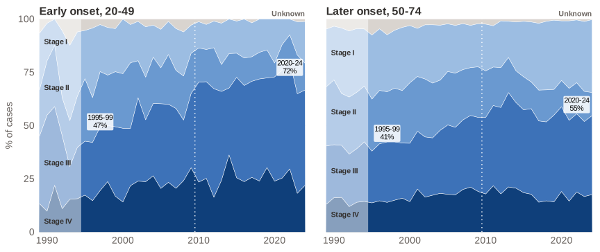
#   incidence   NKR-cijfers (IKNL), the public front end of the Netherlands
#               Cancer Registry: cases by year x sex x 5-year age group, for
#               colon, appendix and rectum separately, and for the
#               gastrointestinal neuroendocrine tumours (NETs), which NKR
#               counts as a group of their own; and by stage, for colon and
#               rectum together and apart (blog: apart is not in the report)
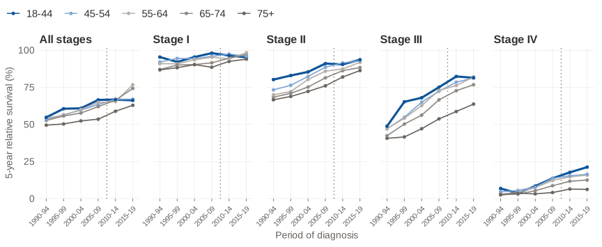
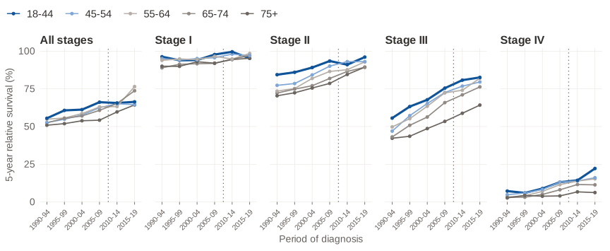
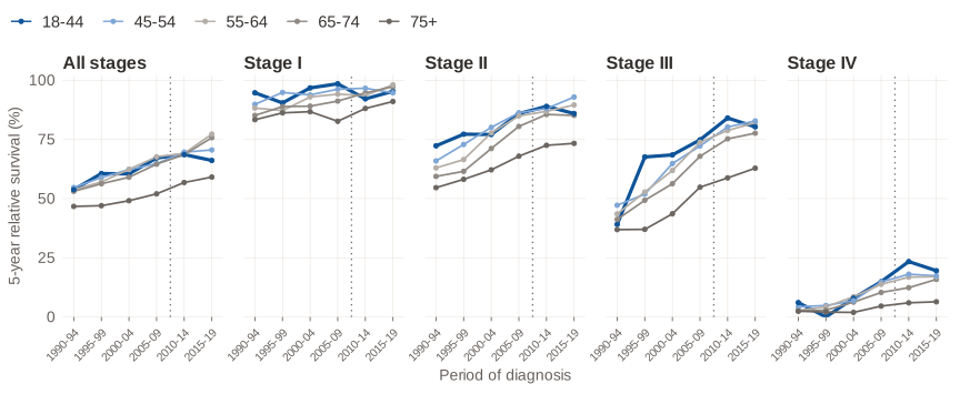
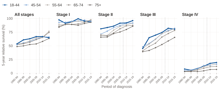
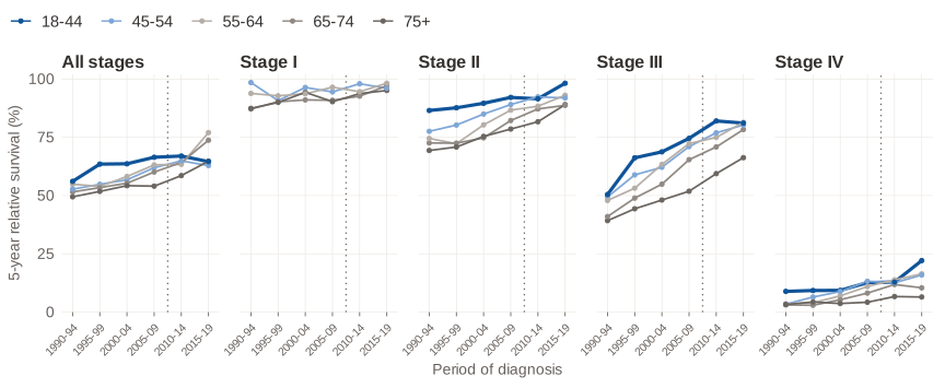
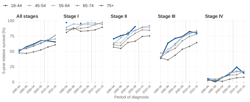
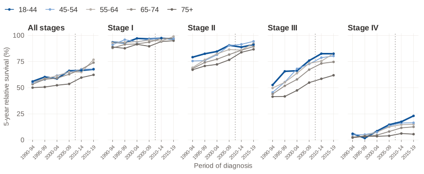
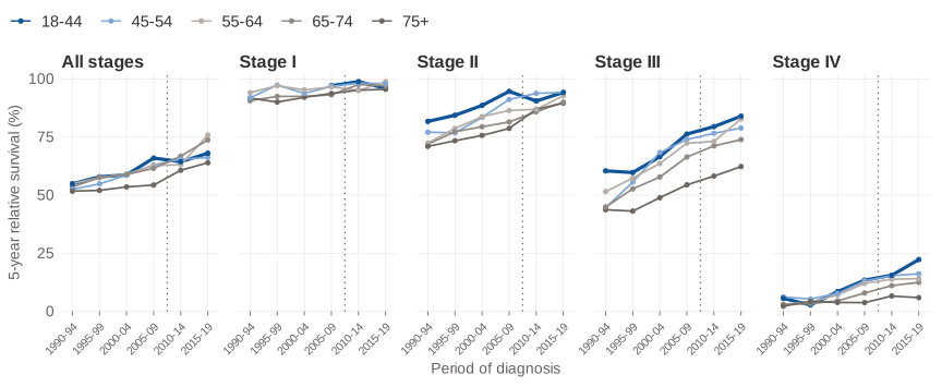
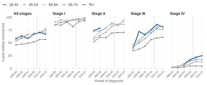
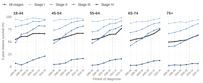
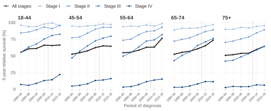
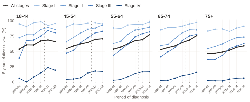
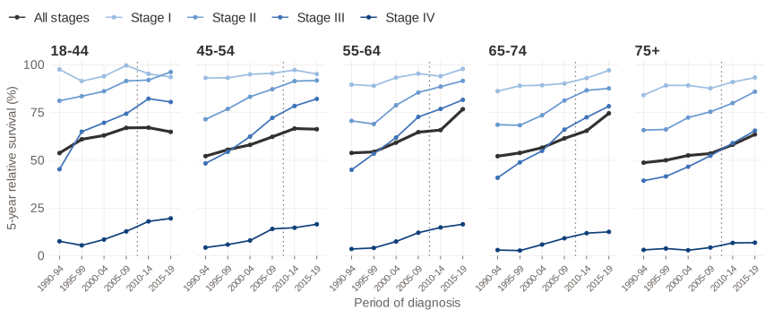
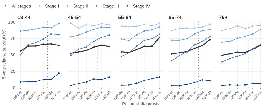
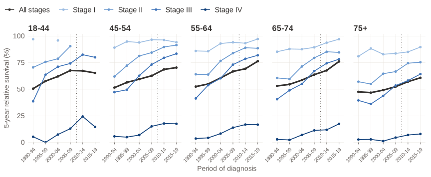
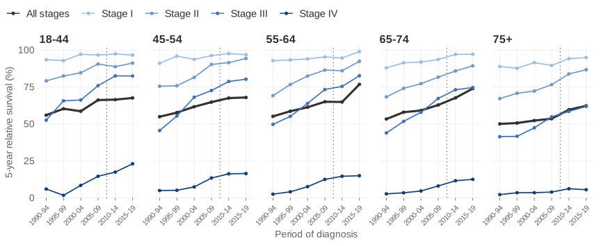
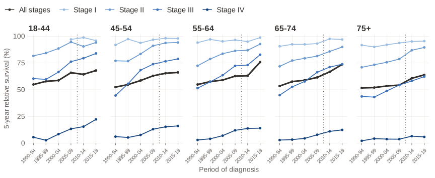
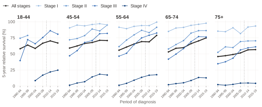
#   survival    NKR-cijfers again (blog: not in the report): relative survival
#               of colon and rectum, together and apart, by 5-year period x
#               NKR's age group x stage
#   mortality   WHO Mortality Database, the Netherlands (4210): deaths by
#               underlying cause at four ICD-10 characters, as CBS reports them,
#               and the C26 deaths (digestive organs, ill-defined) beside them
#   population  CBS StatLine 03759ned: the population on 1 January by sex and
#               single year of age, averaged over 1 January of the year and of
#               the next -- ONE denominator for both outcomes
#
# Each source is fetched as far back as it goes, from NL_FIRST_YEAR at the
# earliest: NKR from 1989, WHO's ICD-10 deaths from 1996, CBS from 1988.
#
# Expects, from the setup chunk:
#   N_AGEGRP, sex_labels, NL_FIRST_YEAR, NKR_KEEP_PRELIMINARY, ua_handle()
# Leaves behind:
#   nl_nkr       the NKR extract: `nkr`, cases per year x sex x agegrp x code
#                with a `preliminary` flag on the years NKR calls provisional;
#                `net`, the same for the GI NETs; and `published`, NKR's own
#                series, kept only to check against
#   nl_stage     `stage`, per site (colon and rectum, appendix excluded; colon;
#                rectum) x year x sex x agegrp x stage, with NKR's suppressed
#                rows as NA (see nkr_stage_cells)
#   nl_surv      `survival`, per site as `stage`, for both sexes and per sex:
#                relative survival in % per period x years after diagnosis x
#                age x stage, with the patients still at risk; cells NKR hides
#                as NA (see nkr_fetch_survival)
#   nl_who       the WHO extract: `deaths`, WHO's own population, unknown ages,
#                and `c26`, the C26 deaths -- NOT part of mort_codes
#   nl_cbs       `cbs_pop`, the CBS population on the 18 bands
#   inc_codes, mort_codes   the two count tables, one row per year x sex x
#                agegrp x code, with the CBS population beside each count
#   net_codes    the GI NETs in the same shape, code "NET (GI)" -- NOT part of
#                inc_codes
#   c26_codes    the C26 deaths in the same shape -- NOT part of mort_codes
# Each of the three extracts carries `fetched`, the day it was downloaded.
# Touches on disk:
#   data/*.parquet, next to this file -- per source: a source whose files are
#   all present, and were fetched from the same NL_FIRST_YEAR, is read; any
#   other is downloaded again and rewritten. Delete one source's files to
#   refresh that source alone.
#
# Every call is namespace-qualified, so nothing has to be attached first.

stopifnot(
  "nl-data.R expects the setup chunk's constants (N_AGEGRP, sex_labels, NL_FIRST_YEAR, NKR_KEEP_PRELIMINARY, ua_handle)" =
    all(vapply(c("N_AGEGRP", "sex_labels", "NL_FIRST_YEAR",
                 "NKR_KEEP_PRELIMINARY", "ua_handle"),
               \(n) exists(n, inherits = TRUE), logical(1))))

# ---- where the extracts are kept ---------------------------------------------
# Parquet, gzip: nanoparquet 0.5.0 accepts "zstd" and then writes the file
# uncompressed.
# blog: in the post's own folder -- Quarto runs the post from there -- rather
# than in the report repository's data/netherlands.
NL_DIR   <- "data"
NL_CACHE <- list(
  nkr = c(nkr       = file.path(NL_DIR, "nkr_incidence.parquet"),
          net       = file.path(NL_DIR, "nkr_net.parquet"),
          published = file.path(NL_DIR, "nkr_published.parquet")),
  # blog: stage and survival per site, each a source of its own, so fetching
  # them did not re-fetch the incidence
  stage = c(stage = file.path(NL_DIR, "nkr_stage_sites.parquet")),
  surv = c(survival = file.path(NL_DIR, "nkr_survival_sites_sexes.parquet")),
  who = c(deaths    = file.path(NL_DIR, "who_nl_deaths.parquet"),
          who_pop   = file.path(NL_DIR, "who_nl_pop.parquet"),
          unknown   = file.path(NL_DIR, "who_nl_unknown_age.parquet"),
          c26       = file.path(NL_DIR, "who_nl_c26.parquet")),
  cbs = c(cbs_pop   = file.path(NL_DIR, "cbs_population.parquet")))

# One source's tables: read them if every file is there and was fetched from
# the NL_FIRST_YEAR asked for now, otherwise run `fetch` and write what it
# returns. all(), not any(): a half-written source must re-fetch rather than
# read the part of itself that happens to be on disk. The day of the download
# and the first year ride in the first file's key-value metadata, as the WHO
# cache does it, rather than as columns repeated on every row.
nl_cached <- function(source, fetch) {
  files <- NL_CACHE[[source]]
  if (all(file.exists(files))) {
    kv <- nanoparquet::read_parquet_metadata(
      files[[1]])$file_meta_data$key_value_metadata[[1]]
    meta <- \(k) kv$value[kv$key == k]
    if (identical(meta("first_year"), as.character(NL_FIRST_YEAR))) {
      out <- lapply(files, \(f) tibble::as_tibble(nanoparquet::read_parquet(f)))
      out$fetched <- as.Date(meta("fetched"))
      return(out)
    }
  }
  out <- fetch()
  dir.create(NL_DIR, showWarnings = FALSE, recursive = TRUE)
  for (nm in names(files))
    nanoparquet::write_parquet(
      out[[nm]], files[[nm]], compression = "gzip",
      metadata = if (nm == names(files)[1])
        c(fetched = as.character(Sys.Date()), first_year = as.character(NL_FIRST_YEAR)))
  out$fetched <- Sys.Date()
  out
}

# ---- NKR-cijfers ---------------------------------------------------------------
# The site runs on an undocumented JSON API.
# blog: found by reading the site's JavaScript bundle. Two endpoints, both POST:
# `filter-groups` lists every filter and its codes, `data` returns the cells.
NKR_API <- "https://api.nkr-cijfers.iknl.nl/api"

# NKR's cancer types and the ICD-10 codes they stand for. NKR classifies a
# tumour on site AND morphology, and keeps the gastrointestinal neuroendocrine
# tumours in a group of their own (subgroep/220000), so each of these three is
# the non-NET tumours of its site. That the rectum is C19-C20 and not C20 alone
# was checked against CI5 XII, whose rectum is C19-C20 by definition: for
# 2013-2017 the two differ by 2% (23,600 against 23,141). Among the Dutch
# deaths of those years C19 is about one in ten of C19-C20, so a rectum
# without it would sit well below CI5's.
#
# The `code` column is what the rest of the post reads. The appendix is
# labelled C181 on purpose -- APPENDIX in the setup chunk -- so it is taken out
# the same way in the cases and in the deaths; the other two carry labels that
# say what they hold rather than pretending to be a single ICD-10 code.
NKR_SITES <- tibble::tribble(
  ~nkr_code,             ~code,            ~nkr_label,
  "kankersoort/205310",  "C18 excl. C181", "Dikkedarmkanker",
  "kankersoort/205320",  "C181",           "Appendixkanker",
  "kankersoort/205330",  "C19-C20",        "Endeldarmkanker")

# The NETs: every site of the digestive tract in one group, which NKR does not
# split by site -- stomach, small bowel, appendix, colon and rectum alike.
NKR_NET <- tibble::tibble(nkr_code = "kankersoort/subgroep/220000",
                          code = "NET (GI)",
                          nkr_label = "Gastrointestinale neuroendocriene tumoren")

NKR_SEXES <- c("geslacht/man" = "Men", "geslacht/vrouw" = "Women")

# The 18 five-year bands, in agegrp order: "00-04jr" .. "80-84jr", then "85-".
NKR_AGES <- c(sprintf("leeftijdsgroep/5-jaar/%02d-%02djr",
                      seq(0, 80, 5), seq(4, 84, 5)),
              "leeftijdsgroep/5-jaar/85-")

nkr_post <- function(path, body) {
  h <- ua_handle()
  curl::handle_setheaders(h, "Content-Type" = "application/json")
  curl::handle_setopt(h, postfields = as.character(
    jsonlite::toJSON(body, auto_unbox = TRUE)))
  res <- curl::curl_fetch_memory(paste0(NKR_API, "/", path, "?format=json"),
                                 handle = h)
  if (res$status_code != 200)
    stop("NKR-cijfers answered ", res$status_code, " on ", path)
  jsonlite::fromJSON(rawToChar(res$content), simplifyVector = FALSE)
}

# Values held fixed in every request: the whole country, every stage.
nkr_fixed <- function(...) c(
  list(...),
  list(list(code = "filter/regio",  values = list(list(code = "regio/totaal/alle"))),
       list(code = "filter/stadium", values = list(list(code = "stadium/totaal/alle")))))

nkr_values <- function(codes) lapply(codes, \(x) list(code = x))

# Which years a page has, and which of them NKR calls provisional -- read off
# the year filter's own remarks, so the flag follows NKR when a year is
# finalised rather than being a year typed in here.
nkr_years <- function(navigation = "incidentie/periode",
                      filter = "filter/periode-van-diagnose") {
  fg <- nkr_post("filter-groups", list(
    currentNavigation = list(code = navigation), language = "nl-NL",
    filterValuesSelected = list(), userAction = list(code = "restart", value = "")))
  flt <- purrr::keep(purrr::list_flatten(purrr::map(fg$filterGroups, "filters")),
                     \(f) identical(f$code, filter))
  stopifnot("NKR-cijfers has no such year filter on that page" = length(flt) == 1)
  leaves <- function(v) purrr::list_flatten(purrr::map(v, \(x)
    if (length(x$children)) leaves(x$children) else list(x)))
  purrr::map(leaves(flt[[1]]$values), \(x) tibble::tibble(
    year = as.integer(sub(".*/", "", x$code)),
    preliminary = any(purrr::map_chr(x$remarks, "code") == "data/preliminary"))) |>
    purrr::list_rbind()
}

# One request per site x sex: every year by every age group. A cell comes back
# with a `state`; anything other than "data/valid" would be a cell NKR has
# suppressed or flagged, and is stopped on below rather than read as a count.
nkr_cells <- function(site, sex, years) {
  d <- nkr_post("data", list(
    language = "nl-NL", navigation = list(code = "incidentie/periode"),
    statistic = list(code = "statistiek/aantal"),
    groupBy = list(
      list(code = "filter/periode-van-diagnose",
           values = nkr_values(paste0("periode/1-jaar/", years))),
      list(code = "filter/leeftijdsgroep", values = nkr_values(NKR_AGES))),
    aggregateBy = nkr_fixed(
      list(code = "filter/kankersoort", values = nkr_values(site)),
      list(code = "filter/geslacht",    values = nkr_values(sex)))))$data
  purrr::map(d, \(r) {
    fv <- purrr::map_chr(r$filterValues, "code")
    tibble::tibble(year   = as.integer(sub(".*/", "", fv[startsWith(fv, "periode/")])),
                   agegrp = match(fv[startsWith(fv, "leeftijdsgroep/")], NKR_AGES),
                   cases  = r$value %||% NA_real_,
                   state  = r$state %||% NA_character_)
  }) |>
    purrr::list_rbind() |>
    dplyr::mutate(nkr_code = site, sex = NKR_SEXES[[sex]])
}

# The same site x sex at all ages, one number per year: what the age groups
# above must add up to. A registry that rounded or perturbed small cells would
# fail this, so it is the check that the counts are counts.
nkr_totals <- function(site, sex, years) {
  d <- nkr_post("data", list(
    language = "nl-NL", navigation = list(code = "incidentie/periode"),
    statistic = list(code = "statistiek/aantal"),
    groupBy = list(list(code = "filter/periode-van-diagnose",
                        values = nkr_values(paste0("periode/1-jaar/", years)))),
    aggregateBy = nkr_fixed(
      list(code = "filter/kankersoort",    values = nkr_values(site)),
      list(code = "filter/geslacht",       values = nkr_values(sex)),
      list(code = "filter/leeftijdsgroep", values = nkr_values("leeftijdsgroep/totaal/alle")))))$data
  purrr::map(d, \(r) tibble::tibble(
    year  = as.integer(sub(".*/", "", purrr::map_chr(r$filterValues, "code"))),
    total = r$value %||% NA_real_)) |>
    purrr::list_rbind() |>
    dplyr::mutate(nkr_code = site, sex = NKR_SEXES[[sex]])
}

# NKR's own published numbers, fetched only to be checked against: the world
# (Segi) standardised incidence rate of all colorectal cancer, persons, and the
# colorectal deaths NKR shows from the CBS cause-of-death statistics.
nkr_published <- function(years) {
  wsr <- nkr_post("data", list(
    language = "nl-NL", navigation = list(code = "incidentie/periode"),
    statistic = list(code = "statistiek/wsr"),
    groupBy = list(list(code = "filter/periode-van-diagnose",
                        values = nkr_values(paste0("periode/1-jaar/", years)))),
    aggregateBy = nkr_fixed(
      list(code = "filter/kankersoort",    values = nkr_values("kankersoort/subgroep/205000")),
      list(code = "filter/geslacht",       values = nkr_values("geslacht/totaal/alle")),
      list(code = "filter/leeftijdsgroep", values = nkr_values("leeftijdsgroep/totaal/alle")))))$data
  # Deaths: CBS splits colorectal into C18 with the appendix, C20 and C19, and
  # its years run on their own calendar, so they are asked for, not assumed.
  dy <- nkr_years("sterfte/periode", "filter/jaar-van-overlijden")
  death_years <- dy$year[dy$year >= NL_FIRST_YEAR]
  deaths <- nkr_post("data", list(
    language = "nl-NL", navigation = list(code = "sterfte/periode"),
    statistic = list(code = "statistiek/aantal"),
    groupBy = list(
      list(code = "filter/jaar-van-overlijden",
           values = nkr_values(paste0("periode/1-jaar/", death_years))),
      list(code = "filter/kankersoortCBS",
           values = nkr_values(paste0("kankersoortCBS/", c("205310", "205330", "205340"))))),
    aggregateBy = list(
      list(code = "filter/geslacht",       values = nkr_values("geslacht/totaal/alle")),
      list(code = "filter/leeftijdsgroep", values = nkr_values("leeftijdsgroep/totaal/alle")))))$data
  year_of <- \(r) as.integer(sub(".*/", "", purrr::keep(
    purrr::map_chr(r$filterValues, "code"), \(x) startsWith(x, "periode/"))))
  dplyr::bind_rows(
    purrr::map(wsr, \(r) tibble::tibble(
      measure = "incidence WSR, C18-C20, persons", year = year_of(r),
      value = r$value %||% NA_real_)) |> purrr::list_rbind(),
    purrr::map(deaths, \(r) tibble::tibble(
      measure = "deaths, C18-C20 (CBS)", year = year_of(r),
      value = r$value %||% NA_real_)) |> purrr::list_rbind() |>
      dplyr::summarise(value = sum(value), .by = c(measure, year)))
}

# Every cell of a set of NKR groups, held to the checks: valid, present, whole,
# and adding up to NKR's own all-ages totals.
nkr_fetch_groups <- function(groups, yrs) {
  years <- yrs$year
  grid  <- tidyr::expand_grid(site = groups$nkr_code, sex = names(NKR_SEXES))

  cells  <- purrr::pmap(grid, \(site, sex) nkr_cells(site, sex, years)) |>
    purrr::list_rbind()
  totals <- purrr::pmap(grid, \(site, sex) nkr_totals(site, sex, years)) |>
    purrr::list_rbind()

  stopifnot(
    "an NKR cell is not marked valid (suppressed or flagged?)" =
      all(cells$state == "data/valid"),
    "an NKR cell came back without a number" = !anyNA(cells$cases),
    "an NKR age group did not match one of the 18 bands" = !anyNA(cells$agegrp),
    # every site x sex x year x band, once
    "NKR did not return the full year x age grid" =
      nrow(cells) == nrow(grid) * length(years) * N_AGEGRP &&
      nrow(dplyr::distinct(cells, nkr_code, sex, year, agegrp)) == nrow(cells),
    "an NKR count is not a whole number" = all(cells$cases == round(cells$cases)))

  gap <- cells |>
    dplyr::summarise(by_age = sum(cases), .by = c(nkr_code, sex, year)) |>
    dplyr::full_join(totals, by = c("nkr_code", "sex", "year"))
  stopifnot("NKR's age groups do not add up to its all-ages total" =
              isTRUE(all(gap$by_age == gap$total)))

  cells |>
    dplyr::inner_join(groups, by = "nkr_code") |>
    dplyr::left_join(yrs, by = "year") |>
    dplyr::transmute(year, preliminary, sex, agegrp = as.integer(agegrp),
                     code, cases)
}

# ---- stage --------------------------------------------------------------------
# Colon and rectum together (NKR sums the two codes when both are in
# aggregateBy), so the appendix is out, as in the main incidence; and, blog:
# colon and rectum apart. Together is asked for rather than added up from the
# two: NKR hides a row by its own size, so the sum of two rows it shows can
# be a row it would show, while either part alone is hidden. Per sex, because
# Persons is built from the sexes, as everywhere else.
#
# The stage is "stage at diagnosis, by the classification valid at the time"
# (NKR-cijfers' own description of the filter): the TNM edition in force in the
# year of diagnosis, pathological stage first and clinical where that is missing
# (Brouwer et al., Int J Cancer 2018). Stage 0 is non-invasive and NVT "no stage
# classification"; both are asked for so the check below sees every case.
NKR_STAGES <- c("stadium/0" = "0", "stadium/i" = "I", "stadium/ii" = "II",
                "stadium/iii" = "III", "stadium/iv" = "IV",
                "stadium/x" = "Unknown", "stadium/nvt" = "NVT")

# NKR hides small cells. In this table it hides WHOLE ROWS -- every stage of one
# year x sex x age group at once, roughly when that row holds 10 cases or fewer
# -- and a hidden row comes back as "data/undisclosed" with no value. Those
# cells are kept as NA rather than worked out from the totals.
# blog: the post uses stage from 20-24 up, and fills in the hidden rows itself
# (the `stage` chunk of index.qmd).
# The provisional year is not asked for; NKR discloses no stage for it.
# blog: the sites, by their NKR codes and the codes of the incidence counts
# their stages must add up to.
NKR_STAGE_SITES <- list(
  `Colon and rectum` = c("kankersoort/205310", "kankersoort/205330"),
  Colon              = "kankersoort/205310",
  Rectum             = "kankersoort/205330")
nkr_site_codes <- \(site) NKR_SITES$code[match(NKR_STAGE_SITES[[site]], NKR_SITES$nkr_code)]

nkr_stage_cells <- function(site, sex, years) {
  d <- nkr_post("data", list(
    language = "nl-NL", navigation = list(code = "incidentie/periode"),
    statistic = list(code = "statistiek/aantal"),
    groupBy = list(
      list(code = "filter/periode-van-diagnose",
           values = nkr_values(paste0("periode/1-jaar/", years))),
      list(code = "filter/leeftijdsgroep", values = nkr_values(NKR_AGES)),
      list(code = "filter/stadium", values = nkr_values(names(NKR_STAGES)))),
    aggregateBy = list(
      list(code = "filter/kankersoort", values = nkr_values(NKR_STAGE_SITES[[site]])),
      list(code = "filter/geslacht", values = nkr_values(sex)),
      list(code = "filter/regio",    values = nkr_values("regio/totaal/alle")))))$data
  purrr::map(d, \(r) {
    fv <- purrr::map_chr(r$filterValues, "code")
    tibble::tibble(year   = as.integer(sub(".*/", "", fv[startsWith(fv, "periode/")])),
                   agegrp = match(fv[startsWith(fv, "leeftijdsgroep/")], NKR_AGES),
                   stage  = unname(NKR_STAGES[fv[startsWith(fv, "stadium/")]]),
                   cases  = r$value %||% NA_real_,
                   state  = r$state %||% NA_character_)
  }) |>
    purrr::list_rbind() |>
    dplyr::mutate(site = site, sex = NKR_SEXES[[sex]])
}

nkr_fetch_stage <- function(yrs, cases) {
  years <- yrs$year[!yrs$preliminary]
  cells <- tidyr::expand_grid(site = names(NKR_STAGE_SITES), sex = names(NKR_SEXES)) |>
    purrr::pmap(\(site, sex) nkr_stage_cells(site, sex, years)) |>
    purrr::list_rbind()

  totals <- purrr::map(names(NKR_STAGE_SITES), \(site) cases |>
    dplyr::filter(code %in% nkr_site_codes(site)) |>
    dplyr::summarise(total = sum(cases), .by = c(year, sex, agegrp)) |>
    dplyr::mutate(site = site)) |>
    purrr::list_rbind()
  rows <- cells |>
    dplyr::summarise(disclosed = all(state == "data/valid"),
                     hidden    = all(state == "data/undisclosed"),
                     by_stage  = sum(cases),
                     .by = c(site, year, sex, agegrp)) |>
    dplyr::left_join(totals, by = c("site", "year", "sex", "agegrp"))

  stopifnot(
    "an NKR stage cell is neither valid nor undisclosed" =
      all(cells$state %in% c("data/valid", "data/undisclosed")),
    "NKR did not return the full year x age x stage grid" =
      nrow(cells) == length(NKR_STAGE_SITES) * length(NKR_SEXES) * length(years) *
        N_AGEGRP * length(NKR_STAGES),
    "an NKR stage row is partly hidden; the post assumes whole rows" =
      all(rows$disclosed | rows$hidden),
    "a valid NKR stage cell came back without a number" =
      !anyNA(cells$cases[cells$state == "data/valid"]),
    # every disclosed row must hold exactly the cases of its site in the main
    # table, so stage splits the incidence the post already uses
    "NKR's stages do not add up to its cases of the site" =
      isTRUE(all(rows$by_stage[rows$disclosed] == rows$total[rows$disclosed])))

  cells |> dplyr::transmute(site, year, sex, agegrp = as.integer(agegrp), stage, cases)
}

fetch_nkr <- function() {
  yrs <- nkr_years() |> dplyr::filter(year >= NL_FIRST_YEAR)
  list(nkr       = nkr_fetch_groups(NKR_SITES, yrs),
       net       = nkr_fetch_groups(NKR_NET, yrs),
       published = nkr_published(yrs$year))
}

# ---- survival -----------------------------------------------------------------
# blog: not in the report. Relative survival per site, as for stage (colon and
# rectum together, so the appendix is out as in the incidence; colon; rectum),
# for both sexes and per sex, per 5-year period of diagnosis from 1990-94 (as
# the post's age-specific rates) x age x stage. Both sexes is NKR's own figure,
# not built from the sexes: relative survival does not add up.
#
# The survival page has age groups of its own (the ICSS groups, 18-44 .. 75+)
# and refuses the 5-year bands. And NKR builds a survival figure from the years
# after diagnosis it is asked for, multiplying their yearly survival: ask for
# year 5 alone and the answer is survival from year 4 to year 5. So every year
# from 0 is asked for, and year k is then k-year survival. The unknown stage is
# not asked for: NKR discloses most of its cells only in part.
NKR_SURV_AGES <- c("leeftijdsgroep/ICSS/18-44jr" = "18-44",
                   "leeftijdsgroep/ICSS/45-54jr" = "45-54",
                   "leeftijdsgroep/ICSS/55-64jr" = "55-64",
                   "leeftijdsgroep/ICSS/65-74jr" = "65-74",
                   "leeftijdsgroep/ICSS/75-"     = "75+")
NKR_SURV_STAGES <- c("stadium/totaal/alle" = "All", "stadium/i" = "I",
                     "stadium/ii" = "II", "stadium/iii" = "III", "stadium/iv" = "IV")
NKR_SURV_YEARS  <- 0:5

NKR_SURV_SEXES <- c("geslacht/totaal/alle" = "Persons", NKR_SEXES)

nkr_fetch_survival <- function(site, sex) {
  periods <- seq(1990L, 2020L, 5L)
  d <- nkr_post("data", list(
    language = "nl-NL", navigation = list(code = "overleving/periode"),
    statistic = list(code = "statistiek/relatieve-overleving"),
    groupBy = list(
      list(code = "filter/periode-van-diagnose",
           values = nkr_values(sprintf("periode/5-jaar/%d-%d", periods, periods + 4L))),
      list(code = "filter/jaren-na-diagnose",
           values = nkr_values(paste0("jaren-na-diagnose/", NKR_SURV_YEARS))),
      list(code = "filter/leeftijdsgroep", values = nkr_values(names(NKR_SURV_AGES))),
      list(code = "filter/stadium",        values = nkr_values(names(NKR_SURV_STAGES)))),
    aggregateBy = list(
      list(code = "filter/kankersoort", values = nkr_values(NKR_STAGE_SITES[[site]])),
      list(code = "filter/geslacht", values = nkr_values(sex)))))$data
  cells <- purrr::map(d, \(r) {
    fv <- purrr::set_names(purrr::map_chr(r$filterValues, "code"),
                           purrr::map_chr(r$filterValues, "filterCode"))
    n <- purrr::keep(r$metaData, \(m) identical(m$code, "metadata/number-of-patients"))
    tibble::tibble(
      period   = as.integer(substr(sub(".*/", "", fv[["filter/periode-van-diagnose"]]), 1, 4)),
      years    = as.integer(sub(".*/", "", fv[["filter/jaren-na-diagnose"]])),
      age      = unname(NKR_SURV_AGES[fv[["filter/leeftijdsgroep"]]]),
      stage    = unname(NKR_SURV_STAGES[fv[["filter/stadium"]]]),
      survival = r$value %||% NA_real_,
      at_risk  = if (length(n)) n[[1]]$value else NA_real_,
      state    = r$state %||% NA_character_)
  }) |>
    purrr::list_rbind()

  # blog: per site and sex the NKR hides some cells -- small groups, such as
  # the rectum at 18-44, stage II, 2020-24 -- whole, at every year after
  # diagnosis; they are kept as NA, and the post decides what to do with them.
  valid <- cells$state == "data/valid"
  stopifnot(
    "an NKR survival cell is neither valid nor undisclosed" =
      all(cells$state %in% c("data/valid", "data/undisclosed")),
    "NKR did not return the full period x years x age x stage grid" =
      nrow(cells) == length(periods) * length(NKR_SURV_YEARS) *
        length(NKR_SURV_AGES) * length(NKR_SURV_STAGES) &&
      nrow(dplyr::distinct(cells, period, years, age, stage)) == nrow(cells),
    "a valid NKR survival cell came back without a number" =
      !anyNA(cells$survival[valid]) && !anyNA(cells$at_risk[valid]),
    # the check that year k is k-year survival, not the survival of year k alone
    "NKR's survival at diagnosis is not 100%" =
      isTRUE(all.equal(cells$survival[valid & cells$years == 0],
                       rep(100, sum(valid & cells$years == 0)))))

  cells |>
    dplyr::select(-state) |>
    dplyr::mutate(site = site, sex = NKR_SURV_SEXES[[sex]], .before = 1)
}

# ---- WHO: the Netherlands ------------------------------------------------------
# blog: WHO's raw ICD-10 mortality files, cut down to one country.
WHO_BASE <- paste0("https://cdn.who.int/media/docs/default-source/",
                   "world-health-data-platform/mortality-raw-data")
WHO_NL   <- "4210"

# The twelve codes a four-character country-year reports for C18-C20. WHO
# leaves a row out when a cause had no deaths, so the grid is completed against
# this set rather than against whatever rows happen to exist.
WHO_CODES <- c(sprintf("C18%d", 0:9), "C19", "C20")

# WHO's lists that code at four characters. The Netherlands filed its first
# ICD-10 years, 1996-1999, on "10M" and every year since on "104"; both carry
# C18.0-C18.9, which is what is checked below rather than taken from the name.
WHO_DETAILED <- c("104", "10M")

# Deaths1..Deaths26 / Pop1..Pop26 -> the 18 bands:
# slot 1 is the all-ages total and 26 is age unknown, neither of them a band;
# 2..6 fold into 0-4 and 23..25 into 85+, which makes every age format WHO uses
# collapse to the same 18 bands.
BAND_MAP <- c(stats::setNames(rep(1L, 5), 2:6),
              stats::setNames(2:17,       7:22),
              stats::setNames(rep(18L, 3), 23:25))

fetch_who_nl <- function() {
  tmp <- tempfile("who"); dir.create(tmp)
  get_one <- function(name) {
    zip <- file.path(tmp, paste0(name, ".zip"))
    curl::curl_download(paste0(WHO_BASE, "/", name, ".zip"), zip, quiet = TRUE,
                        handle = ua_handle())
    utils::unzip(zip, exdir = tmp)
  }
  purrr::walk(c(paste0("morticd10_part", 1:6), "mort_pop"), get_one)
  parts <- file.path(tmp, paste0("Morticd10_part", 1:6))
  pop_f <- file.path(tmp, "pop")
  stopifnot("a WHO archive does not hold the file this reader expects" =
              all(file.exists(c(parts, pop_f))))

  # One country out of ~500 MB: keep its lines as text first and parse only
  # those, rather than parsing every country to throw all but one away.
  read_country <- function(f) {
    x <- readr::read_lines(f, progress = FALSE)
    readr::read_csv(I(c(x[1], x[startsWith(x, paste0(WHO_NL, ","))])),
                    col_types = readr::cols(.default = readr::col_character()),
                    progress = FALSE)
  }

  all_nl <- purrr::map(parts, read_country) |>
    purrr::list_rbind() |>
    dplyr::mutate(Year = as.integer(Year)) |>
    dplyr::filter(Year >= NL_FIRST_YEAR)

  raw <- all_nl |> dplyr::filter(stringr::str_detect(Cause, "^C1[89]|^C20"))

  # Every year used must code C18 at four characters: that is what makes the
  # twelve codes the vocabulary, and what lets the appendix (C18.1) be taken
  # out at all. A three-character C18 anywhere would break both.
  stopifnot(
    "a Dutch WHO year is on a list that does not code at four characters" =
      all(raw$List %in% WHO_DETAILED),
    "a Dutch WHO year reports a three-character C18" = !any(raw$Cause == "C18"),
    "a Dutch WHO colorectal code is outside the twelve expected" =
      all(raw$Cause %in% WHO_CODES),
    "a Dutch WHO year is missing in the middle of the series" =
      all(seq(min(raw$Year), max(raw$Year)) %in% raw$Year),
    "WHO has a Dutch death of a sex other than 1/2" = all(raw$Sex %in% c("1", "2")))

  long <- raw |>
    tidyr::pivot_longer(
      tidyselect::matches("^Deaths([2-9]|1[0-9]|2[0-6])$"),
      names_to = "slot", values_to = "deaths",
      names_transform = list(slot = \(x) as.integer(sub("Deaths", "", x)))) |>
    dplyr::mutate(deaths = tidyr::replace_na(as.numeric(deaths), 0))

  stopifnot("WHO age bands do not sum to the published all-ages total" =
              isTRUE(all.equal(sum(long$deaths),
                               sum(as.numeric(raw$Deaths1), na.rm = TRUE))))

  deaths <- long |>
    dplyr::filter(slot %in% as.integer(names(BAND_MAP))) |>
    dplyr::transmute(year = Year, list = List,
                     sex = sex_labels[as.integer(Sex)],
                     agegrp = unname(BAND_MAP[as.character(slot)]),
                     code = Cause, deaths) |>
    dplyr::summarise(deaths = sum(deaths), .by = c(year, list, sex, agegrp, code)) |>
    tidyr::complete(tidyr::nesting(year, list), sex = sex_labels,
                    agegrp = seq_len(N_AGEGRP), code = WHO_CODES,
                    fill = list(deaths = 0))

  unknown <- long |>
    dplyr::filter(slot == 26) |>
    dplyr::summarise(unknown = sum(deaths), .by = Year) |>
    dplyr::rename(year = Year)

  who_pop <- readr::read_csv(pop_f, col_types = readr::cols(.default = readr::col_character()),
                             progress = FALSE) |>
    dplyr::filter(Country == WHO_NL, Sex %in% c("1", "2")) |>
    dplyr::mutate(Year = as.integer(Year)) |>
    dplyr::filter(Year >= NL_FIRST_YEAR) |>
    tidyr::pivot_longer(
      tidyselect::matches("^Pop([2-9]|1[0-9]|2[0-5])$"),
      names_to = "slot", values_to = "pop",
      names_transform = list(slot = \(x) as.integer(sub("Pop", "", x)))) |>
    dplyr::transmute(year = Year, sex = sex_labels[as.integer(Sex)],
                     agegrp = unname(BAND_MAP[as.character(slot)]),
                     pop = tidyr::replace_na(as.numeric(pop), 0)) |>
    dplyr::summarise(pop = sum(pop), .by = c(year, sex, agegrp))

  # C26, "other and ill-defined digestive organs". C26.0 is "intestinal tract,
  # part unspecified", where a death certified only as bowel cancer ends up, so
  # it is the one code outside C18-C20 that may hold colorectal deaths. Kept at
  # whatever detail WHO has, by the same age bands, completed like the deaths.
  death_years <- unique(deaths$year)
  c26 <- all_nl |>
    dplyr::filter(stringr::str_detect(Cause, "^C26"), Sex %in% c("1", "2")) |>
    tidyr::pivot_longer(
      tidyselect::matches("^Deaths([2-9]|1[0-9]|2[0-6])$"),
      names_to = "slot", values_to = "deaths",
      names_transform = list(slot = \(x) as.integer(sub("Deaths", "", x)))) |>
    dplyr::mutate(deaths = tidyr::replace_na(as.numeric(deaths), 0)) |>
    dplyr::filter(slot %in% as.integer(names(BAND_MAP))) |>
    dplyr::transmute(year = Year, sex = sex_labels[as.integer(Sex)],
                     agegrp = unname(BAND_MAP[as.character(slot)]),
                     code = Cause, deaths) |>
    dplyr::summarise(deaths = sum(deaths), .by = c(year, sex, agegrp, code)) |>
    tidyr::complete(year = death_years, sex = sex_labels,
                    agegrp = seq_len(N_AGEGRP), code,
                    fill = list(deaths = 0))

  list(deaths = deaths, who_pop = who_pop, unknown = unknown, c26 = c26)
}

# ---- CBS StatLine: population --------------------------------------------------
# Table 03759ned, through the OData v3 API (no key). The dimension keys are
# padded to a fixed width -- "NL01  ", "3000   " -- and a filter on the bare
# key matches nothing, so the keys are written out padded.
#
# WHICH population. The table offers two, and the obvious one is wrong here.
# Its "gemiddelde bevolking" (average population) at age L is the cohort that
# turns L during the year -- CBS defines it as (aged L-1 on 1 January + aged L
# on 31 December) / 2 -- so its ages run half a year older than the age at
# diagnosis or death that NKR and WHO count. Against those numerators it puts
# too many people in every old band and too few in 0-4, and an all-ages ASR
# comes out about 2% low. The population used instead is the 1 January
# population at age L, averaged over 1 January of the year and of the next:
# the people at that same age at the start and at the end of the year, which
# is what a mid-year population by age is. With it, the Segi ASR of the NKR
# counts reproduces the WSR NKR publishes to within 0.05% in every final year
# (checked October 2026; blog: the check is redone in the post).
# WHO's own Dutch population is this same series too, except around 2018-2020,
# where its split by age departs from it by up to 18% -- so it is kept only for
# that comparison.
CBS_URL <- "https://opendata.cbs.nl/ODataApi/odata/03759ned"

fetch_cbs <- function() {
  get_json <- function(url, query = list()) {
    h <- ua_handle()
    u <- if (length(query)) paste0(url, "?", paste(
      names(query), vapply(query, curl::curl_escape, ""), sep = "=", collapse = "&"))
      else url
    res <- curl::curl_fetch_memory(u, handle = h)
    if (res$status_code != 200) stop("CBS answered ", res$status_code)
    jsonlite::fromJSON(rawToChar(res$content))$value
  }

  ages <- tibble::as_tibble(get_json(paste0(CBS_URL, "/Leeftijd"))) |>
    dplyr::transmute(Leeftijd = trimws(Key), title = Title)

  d <- tibble::as_tibble(get_json(paste0(CBS_URL, "/TypedDataSet"), list(
    `$filter` = paste("RegioS eq 'NL01  ' and BurgerlijkeStaat eq 'T001019'",
                      "and (Geslacht eq '3000   ' or Geslacht eq '4000   ')"),
    `$select` = "Geslacht,Leeftijd,Perioden,BevolkingOp1Januari_1"))) |>
    dplyr::mutate(dplyr::across(c(Geslacht, Leeftijd), trimws),
                  jan1 = as.integer(substr(Perioden, 1, 4))) |>
    # 1 January of the first year is needed, and of the year after the last
    dplyr::filter(jan1 >= NL_FIRST_YEAR, !is.na(BevolkingOp1Januari_1)) |>
    dplyr::left_join(ages, by = "Leeftijd") |>
    dplyr::mutate(sex = dplyr::if_else(Geslacht == "3000", "Men", "Women"),
                  single = suppressWarnings(as.integer(
                    sub("^(\\d+) jaar$", "\\1", title))),
                  pop = BevolkingOp1Januari_1)

  # The table holds single years of age, an all-ages total, AND open bands
  # ("95 jaar of ouder", "105 jaar of ouder") that overlap the single years. So
  # the bands 0-4 .. 80-84 are built from single years 0..84 only, and 85+ is
  # the total minus those -- which does not depend on how CBS happens to split
  # the oldest ages in a given year.
  single <- d |> dplyr::filter(!is.na(single), single <= 84)
  total  <- d |> dplyr::filter(title == "Totaal") |>
    dplyr::select(jan1, sex, total = pop)

  stopifnot(
    "CBS is missing a single year of age below 85" =
      all(dplyr::count(single, jan1, sex)$n == 85L),
    "CBS has no all-ages total for a year" =
      nrow(total) == nrow(dplyr::distinct(single, jan1, sex)))

  bands <- single |>
    dplyr::mutate(agegrp = single %/% 5L + 1L) |>
    dplyr::summarise(pop = sum(pop), .by = c(jan1, sex, agegrp))

  old <- bands |>
    dplyr::summarise(under85 = sum(pop), .by = c(jan1, sex)) |>
    dplyr::inner_join(total, by = c("jan1", "sex")) |>
    dplyr::transmute(jan1, sex, agegrp = N_AGEGRP, pop = total - under85)

  stopifnot("CBS 85+ came out at zero or below" = all(old$pop > 0))

  stocks <- dplyr::bind_rows(bands, old) |> dplyr::mutate(agegrp = as.integer(agegrp))

  # Year t's population is the mean of the stocks on 1 January t and 1 January
  # t+1, at the same age. An inner join, so a year is only produced once the
  # following 1 January is published.
  dplyr::inner_join(
    stocks |> dplyr::rename(year = jan1, start = pop),
    stocks |> dplyr::transmute(year = jan1 - 1L, sex, agegrp, end = pop),
    by = c("year", "sex", "agegrp")) |>
    dplyr::transmute(year, sex, agegrp, pop = (start + end) / 2) |>
    dplyr::arrange(year, sex, agegrp)
}

# ---- read the cache, or build it, one source at a time ----------------------------
nl_nkr <- nl_cached("nkr", fetch_nkr)
nl_stage <- nl_cached("stage", \() list(stage = nkr_fetch_stage(
  nkr_years() |> dplyr::filter(year >= NL_FIRST_YEAR), nl_nkr$nkr)))
nl_surv <- nl_cached("surv", \() list(survival = tidyr::expand_grid(
  site = names(NKR_STAGE_SITES), sex = names(NKR_SURV_SEXES)) |>
  purrr::pmap(nkr_fetch_survival) |>
  purrr::list_rbind()))
nl_who <- nl_cached("who", fetch_who_nl)
nl_cbs <- nl_cached("cbs", \() list(cbs_pop = fetch_cbs()))

stopifnot(
  "CBS bands do not tile 0-85+" =
    all(dplyr::count(nl_cbs$cbs_pop, year, sex)$n == N_AGEGRP),
  "WHO has Dutch deaths of unknown age, which no band would hold" =
    sum(nl_who$unknown$unknown) == 0)

# ---- the count tables, each count with its population ---------------------------
# One row per year x sex x age group x code, rectangular, with `pop` repeated
# across the codes of a cell.
# blog: the report put these in the shape of the ICBP files, with a country and
# jurisdiction column; one country needs neither.
with_pop <- function(d) {
  out <- d |>
    dplyr::left_join(nl_cbs$cbs_pop, by = c("year", "sex", "agegrp")) |>
    dplyr::transmute(year, sex, agegrp = as.integer(agegrp), code, cases, pop)
  stopifnot("a Dutch count has no CBS population under it" = !anyNA(out$pop))
  out
}

keep_final <- \(d) d |>
  dplyr::filter(NKR_KEEP_PRELIMINARY | !preliminary) |>
  dplyr::select(-preliminary)

inc_codes <- nl_nkr$nkr |> keep_final() |> with_pop()
net_codes <- nl_nkr$net |> keep_final() |> with_pop()

mort_codes <- nl_who$deaths |>
  dplyr::select(year, sex, agegrp, code, cases = deaths) |>
  with_pop()

c26_codes <- nl_who$c26 |>
  dplyr::select(year, sex, agegrp, code, cases = deaths) |>
  with_pop()

# Segi (1960) world standard population, per 100,000, for the 18 age groups
SEGI <- c(12000, 10000, 9000, 9000, 8000, 8000, 6000, 6000, 6000, 6000,
          5000, 4000, 4000, 3000, 2000, 1000, 500, 500)
age_label <- \(g) if_else(g == 18, "85+", str_c((g - 1) * 5, "-", (g - 1) * 5 + 4))

# Cases (or deaths) and population per sex, year and age group for a set of
# codes, with Persons added. The codes share a population, so they are summed
# within a sex first; men and women do not, so Persons adds their populations.
by_sex <- function(d, codes = unique(d$code)) {
  s <- d |>
    filter(code %in% codes) |>
    summarise(cases = sum(cases), pop = first(pop), .by = c(sex, year, agegrp))
  bind_rows(s,
            s |>
              summarise(cases = sum(cases), pop = sum(pop), .by = c(year, agegrp)) |>
              mutate(sex = "Persons")) |>
    mutate(sex = factor(sex, SEXES))
}

# The age-standardised rate per 100,000 over the age groups `ages`, per sex
# and year
asr <- function(d, ages) {
  d |>
    filter(agegrp %in% ages) |>
    mutate(w = SEGI[agegrp] / sum(SEGI[ages])) |>
    summarise(rate = sum(w * cases / pop) * 1e5, cases = sum(cases), .by = c(sex, year)) |>
    arrange(sex, year)
}

# Colon and rectum: the NKR's two groups, so the appendix and the NETs are out
CRC <- c("C18 excl. C181", "C19-C20")
inc <- list(
  `Colon and rectum` = by_sex(inc_codes, CRC),
  Colon              = by_sex(inc_codes, "C18 excl. C181"),
  Rectum             = by_sex(inc_codes, "C19-C20"),
  Appendix           = by_sex(inc_codes, APPENDIX),
  NET                = by_sex(net_codes))
mort     <- by_sex(mort_codes |> filter(code != APPENDIX))
# The deaths split as the cases: the colon is C18 without the appendix, the
# rectum C19-C20
SITES  <- c("Colon and rectum", "Colon", "Rectum")
DEATHS <- list(`Colon and rectum` = mort,
               Colon  = by_sex(mort_codes |> filter(str_starts(code, "C18"), code != APPENDIX)),
               Rectum = by_sex(mort_codes |> filter(code %in% c("C19", "C20"))))
mort_c26 <- by_sex(bind_rows(mort_codes |> filter(code != APPENDIX),
                             c26_codes |> filter(code == "C260")))
# The share of those deaths certified as C26.0, over the age groups `ages` and
# the years `years`
c26_share <- function(ages, years) {
  n <- \(d) sum(d$cases[d$agegrp %in% ages & d$year %in% years])
  100 * n(filter(c26_codes, code == "C260")) / n(filter(mort_c26, sex == "Persons"))
}

# A number in the text: rounded, with a thousands separator
fmt <- \(x, digits = 1) formatC(x, format = "f", digits = digits, big.mark = ",")

# The check against the NKR's own world-standardised rate: all ages, both
# sexes, and the appendix in, as in the NKR's own colorectal group
wsr_check <- asr(by_sex(inc_codes), 1:18) |>
  filter(sex == "Persons") |>
  inner_join(nl_nkr$published |>
               filter(measure == "incidence WSR, C18-C20, persons") |>
               select(year, wsr = value), by = "year") |>
  mutate(diff = 100 * (rate / wsr - 1))
wsr_check_max <- max(abs(wsr_check$diff))
stopifnot("the age-standardised rate no longer reproduces the NKR's own to 0.05%" =
            wsr_check_max < 0.05)

Below, I plot the mortality and incidence series for early onset (20-49) and later onset (50-74)³ and estimate the annual percentage change (EAPC) by fitting a straight line through the logarithm of the yearly rates and turning the slope estimate into percentage change per year.

# The EAPC as in my report (and Rcan::csu_eapc): a straight line through the
# log of the yearly rates over the last `n` years of a series, whose slope b
# becomes a percentage change per year, 100 * (exp(b) - 1); the 95% interval
# is b +/- 1.96 standard errors. A year with no cases has no log rate and is
# left out of the fit, and with fewer than three years left there is no fit.
# `keys` are the columns that tell one series from another.
WINDOWS <- c(`Past 10 years` = 10L, `Past 30 years` = 30L)

eapc <- function(d, n, keys = "sex") {
  d |>
    mutate(window_to = max(year), window_from = window_to - n + 1L,
           .by = all_of(keys)) |>
    filter(year >= window_from) |>
    nest(.by = all_of(c(keys, "window_from", "window_to"))) |>
    mutate(years_zero = map_int(data, \(x) sum(x$rate == 0)),
           fit = map(data, \(x) {
             x <- filter(x, rate > 0)
             if (nrow(x) < 3)
               return(tibble(eapc = NA_real_, low = NA_real_, up = NA_real_,
                             intercept = NA_real_, slope = NA_real_,
                             year_from = NA_real_, year_to = NA_real_))
             m  <- summary(lm(log(rate) ~ year, data = x))$coefficients
             b  <- m["year", "Estimate"]
             se <- m["year", "Std. Error"]
             tibble(eapc = 100 * (exp(b) - 1),
                    low  = 100 * (exp(b - qnorm(0.975) * se) - 1),
                    up   = 100 * (exp(b + qnorm(0.975) * se) - 1),
                    intercept = m["(Intercept)", "Estimate"], slope = b,
                    year_from = min(x$year), year_to = max(x$year))
           })) |>
    select(-data) |>
    unnest(fit)
}

# The EAPC of an age-standardised rate over the age groups `ages`, both sexes
# unless asked for one, as it is quoted in the text
band_eapc <- function(d, ages, window, sex = "Persons") {
  eapc(asr(d, ages), WINDOWS[[window]]) |> filter(sex == !!sex)
}
# Numbers in the text: the estimate in bold, its interval not
fmt_eapc <- \(r) sprintf("**%+.1f%%** a year (95%% CI %+.1f to %+.1f)", r$eapc, r$low, r$up)
fmt_e    <- \(r) sprintf("**%+.1f%%**", r$eapc)

BAND_AGES <- list(`Early onset, 20-49` = 5:10, `Later onset, 50-74` = 11:15)

trend <- imap(list(Incidence = inc[SITES], Mortality = DEATHS), \(sites, outcome)
  imap(sites, \(d, site) imap(BAND_AGES, \(a, b) asr(d, a) |> mutate(band = b)) |>
         list_rbind() |> mutate(site = site)) |>
    list_rbind() |> mutate(outcome = outcome)) |>
  list_rbind() |>
  mutate(band = factor(band, names(BAND_AGES)))

trend_fit <- imap(WINDOWS, \(n, w) eapc(trend, n, keys = c("outcome", "site", "band", "sex")) |>
                    mutate(window = w)) |>
  list_rbind()

# A rate in the text: one outcome, band and year, both sexes, colon and rectum
# unless asked for one
trend_at <- function(outcome, band, yr, site = "Colon and rectum") {
  trend$rate[trend$outcome == outcome & trend$band == band & trend$sex == "Persons" &
               trend$site == site & trend$year == yr]
}
trend_eapc <- \(outcome, band, window, sex = "Persons", site = "Colon and rectum") trend_fit |>
  filter(outcome == !!outcome, band == !!band, window == !!window, sex == !!sex,
         site == !!site)

# Two y axes per panel: incidence on the left, mortality on the right. The
# right-hand axis runs to twice the highest death rate of any sex and site, so
# that the deaths run along the lower half of the panel and the cases along
# the upper, and each axis is the same in every tab; `k` turns a death rate into the
# left-hand scale.
nice_top <- \(x) max(pretty(c(0, x)))
AXES <- trend |>
  summarise(top = max(rate), .by = c(outcome, band)) |>
  pivot_wider(names_from = outcome, values_from = top) |>
  mutate(left = map_dbl(Incidence, nice_top), right = map_dbl(2 * Mortality, nice_top),
         k = left / right)

# Annual rates as points joined by a pale line, the trend over the window as a
# dashed line in a darker shade, and its EAPC at the line's end -- as in the
# manuscript's time series. The EAPC label also names its series, in the colour
# of that series' axis, so there is no legend to look up. The start of
# screening is marked where it applies.
# Years on the x axis: the decades, and in smaller type the first and last
# year of the window. A size per label is not officially supported by
# ggplot2, and warns, but works.
# In narrower panels, `gap` leaves out the decades that close to a window year.
window_years <- \(window) max(trend$year) - c(WINDOWS[[window]] - 1L, 0L)
trend_years  <- function(window, gap = 0) {
  w <- window_years(window)
  decades <- seq(1990, max(trend$year), 10)
  sort(c(keep(decades, \(y) all(abs(y - w) > gap)), w))
}

fig_trends <- function(window, sex, site) {
  panels <- map(levels(trend$band), \(b) {
    ax    <- filter(AXES, band == b)
    on_ax <- \(outcome, y) if_else(outcome == "Mortality", y * ax$k, y)
    d   <- trend |>
      filter(band == b, sex == !!sex, site == !!site) |>
      mutate(y = on_ax(outcome, rate))
    fit <- trend_fit |> filter(band == b, sex == !!sex, site == !!site, window == !!window)
    seg <- fit |>
      mutate(year = map2(year_from, year_to, \(a, z) seq(a, z, length.out = 25))) |>
      unnest(year) |>
      mutate(y = on_ax(outcome, exp(intercept + slope * year)))
    lab <- fit |>
      mutate(year = year_to, y = on_ax(outcome, exp(intercept + slope * year_to)),
             label = str_c(outcome, "\n", sprintf("%+.1f%%/yr", eapc)))
    screen <- if (b == "Later onset, 50-74")
      list(geom_vline(xintercept = 2013.5, colour = COL[["context"]], linetype = "dotted",
                      linewidth = 0.45),
           annotate("text", x = 2013.5, y = ax$left, label = "Screening starts\n(FIT, 55-75)",
                    hjust = 1.05, vjust = 1, size = TEXT * 0.9, colour = COL[["context"]],
                    family = FIG_FONT, lineheight = 0.95))

    ggplot(d, aes(year, y, colour = outcome)) +
      screen +
      geom_line(linewidth = 0.4, alpha = 0.35) +
      geom_point(size = 0.9) +
      geom_line(data = seg, aes(colour = str_c(outcome, " trend")), linewidth = 0.8,
                linetype = "62", show.legend = FALSE) +
      # ggrepel: in the rectum the two labels can end at the same height
      ggrepel::geom_text_repel(data = lab, aes(label = label, colour = outcome), hjust = 0,
                               nudge_x = 0.8, direction = "y", xlim = c(max(d$year) + 0.5, Inf),
                               size = TEXT, fontface = "bold", family = FIG_FONT,
                               lineheight = 0.9, segment.colour = NA,
                               min.segment.length = Inf, box.padding = 0.15, seed = 1) +
      scale_colour_manual(
        values = c(COL[c("Incidence", "Mortality")],
                   `Incidence trend` = alpha(shade(COL[["Incidence"]]), 0.85),
                   `Mortality trend` = alpha(shade(COL[["Mortality"]]), 0.85)),
        guide = "none") +
      scale_y_continuous(limits = c(0, ax$left), breaks = pretty(c(0, ax$left)),
                         expand = expansion(mult = c(0, 0.03)),
                         name = "Incidence per 100,000 (age-standardised)",
                         sec.axis = sec_axis(~ . / ax$k, breaks = pretty(c(0, ax$right)),
                                             name = "Mortality per 100,000 (age-standardised)")) +
      scale_x_continuous(breaks = trend_years(window),
                         expand = expansion(add = c(1, 11))) +
      coord_cartesian(clip = "off") +
      labs(title = b, x = NULL) +
      theme_ft("xy") +
      theme(axis.text.x        = element_text(
              size = rel(if_else(trend_years(window) %in% window_years(window), 0.75, 1)),
              vjust = 1),
            axis.ticks.x       = element_line(colour = COL[["axis"]], linewidth = 0.3),
            axis.ticks.length.x = unit(1.2, "mm"),
            axis.text.y.left   = element_text(colour = COL[["Incidence"]]),
            axis.title.y.left  = element_text(colour = COL[["Incidence"]]),
            axis.text.y.right  = element_text(colour = COL[["Mortality"]]),
            axis.title.y.right = element_text(colour = COL[["Mortality"]]))
  })
  wrap_plots(panels, nrow = 1)
}

Past 10 years

Persons

Colon and rectum

Colon

Rectum

Men

Colon and rectum

Colon

Rectum

Women

Colon and rectum

Colon

Rectum

Past 30 years

Persons

Colon and rectum

Colon

Rectum

Men

Colon and rectum

Colon

Rectum

Women

Colon and rectum

Colon

Rectum

As you can see, colorectal carcinomas show very different trends between late and early onset. The rollout of FIT screening (a test for blood in the stool, at 55-75y) at first found many more cancers, after which incidence dropped sharply: screening had brought diagnoses forward, and removed polyps before they could turn into cancer. Early-onset colorectal cancer, on the other hand, is rising, mostly in the colon: there the rise was steeper over the past 10 years than over the past 30, while rectal cancer turned down. Trends also appear to be steeper among men.

Next, let’s look if there’s variation within these age groups.

AGE_GROUPS <- 5:18   # 20-24 ... 85+
FIT_KIND <- c("Every year had cases", "Some years had no cases")

# The cases (or deaths) behind each fit: all of them in the window's years
window_cases <- \(d, n) d |>
  filter(year > max(year) - n) |>
  summarise(cases = sum(cases), .by = c(sex, agegrp))

age_fit <- imap(list(Incidence = inc[SITES], Mortality = DEATHS), \(sites, outcome)
  imap(WINDOWS, \(n, w)
    imap(sites, \(d, site) {
      d <- d |>
        filter(agegrp %in% AGE_GROUPS) |>
        mutate(rate = cases / pop * 1e5)
      eapc(d, n, keys = c("sex", "agegrp")) |>
        left_join(window_cases(d, n), by = c("sex", "agegrp")) |>
        mutate(site = site)
    }) |>
      list_rbind() |>
      mutate(window = w)) |>
    list_rbind() |>
    mutate(outcome = outcome)) |>
  list_rbind() |>
  mutate(site = factor(site, SITES),
         age  = factor(age_label(agegrp), rev(age_label(AGE_GROUPS))),
         fit  = factor(if_else(years_zero > 0, FIT_KIND[2], FIT_KIND[1]), FIT_KIND))

age_eapc_at <- \(site, age, window, sex = "Persons", outcome = "Incidence") age_fit |>
  filter(site == !!site, age == !!age, window == !!window, sex == !!sex,
         outcome == !!outcome)

# The same axis in every tab, so the sexes and the windows compare; an
# interval that runs past it ends in an arrowhead, and an EAPC past it sits on
# its edge with its value written next to it
EAPC_XLIM <- c(-10, 10)

# An age group per row, the youngest at the top; in each row the cases above
# and the deaths below, with their number in the window just right of the
# panel. Each EAPC is written by its point, the cases' above and the deaths'
# below. Dashed lines mark off 20-49 and 50-74. A fit that had to leave out a
# year without a single case is drawn hollow: such fits are pulled toward no
# change, as the years left out are the lowest.
fig_age_eapc <- function(window, sex, site) {
  xlim <- EAPC_XLIM
  d <- age_fit |>
    filter(window == !!window, sex == !!sex, site == !!site, !is.na(eapc)) |>
    mutate(y    = as.integer(age) + if_else(outcome == "Incidence", 0.17, -0.17),
           x    = pmin(pmax(eapc, xlim[1]), xlim[2]),
           lo_c = pmax(low, xlim[1]), hi_c = pmin(up, xlim[2]))
  under50   <- sum(levels(d$age) %in% age_label(5:10))
  over74    <- sum(levels(d$age) %in% age_label(16:N_AGEGRP))
  arrow_end <- arrow(length = unit(1, "mm"), type = "closed", angle = 25)
  whisker   <- \(...) geom_segment(..., linewidth = 0.4)
  off_axis  <- filter(d, abs(eapc) > xlim[2])

  ggplot(d, aes(y = y, colour = outcome)) +
    annotate("segment", x = xlim[1], xend = xlim[2],
             y = c(length(levels(d$age)) - under50, over74) + 0.5,
             colour = COL[["context"]], linewidth = 0.3, linetype = "dashed") +
    geom_vline(xintercept = 0, colour = COL[["ink"]], linewidth = 0.45) +
    whisker(aes(x = x, xend = lo_c, yend = y), data = \(x) filter(x, low >= xlim[1])) +
    whisker(aes(x = x, xend = lo_c, yend = y), data = \(x) filter(x, low < xlim[1], x > lo_c),
            arrow = arrow_end) +
    whisker(aes(x = x, xend = hi_c, yend = y), data = \(x) filter(x, up <= xlim[2])) +
    whisker(aes(x = x, xend = hi_c, yend = y), data = \(x) filter(x, up > xlim[2], x < hi_c),
            arrow = arrow_end) +
    # show.legend = TRUE: without it, a kind of fit the tab does not have gets
    # an empty key
    geom_point(aes(x = x, shape = fit), fill = "white", size = 1.8, stroke = 0.6,
               show.legend = TRUE) +
    geom_text(data = off_axis, aes(x = x, label = sprintf("%+.0f", eapc),
                                   hjust = if_else(eapc > 0, 1, 0)),
              nudge_x = if_else(off_axis$eapc > 0, -0.8, 0.8), size = TEXT * 0.85,
              family = FIG_FONT, show.legend = FALSE) +
    geom_text(aes(x = x, label = sprintf("%+.1f", eapc),
                  vjust = if_else(outcome == "Incidence", -0.9, 1.8)),
              data = \(x) filter(x, abs(eapc) <= xlim[2]), size = TEXT * 0.65,
              family = FIG_FONT, show.legend = FALSE) +
    geom_text(aes(x = xlim[2], label = fmt(cases, 0)), hjust = 0, nudge_x = 0.9,
              size = TEXT * 0.75, family = FIG_FONT, show.legend = FALSE) +
    scale_x_continuous(breaks = seq(xlim[1], xlim[2], 2),
                       labels = \(x) if_else(x > 0, str_c("+", x), as.character(x))) +
    scale_y_continuous(breaks = seq_along(levels(d$age)), labels = if_else(levels(d$age) == "85+", ">84y", str_c(levels(d$age), "y")),
                       expand = expansion(add = 0.6)) +
    scale_colour_manual(values = COL[c("Incidence", "Mortality")]) +
    scale_shape_manual(values = set_names(c(19, 21), FIT_KIND), drop = FALSE) +
    guides(shape = guide_legend(order = 2, override.aes = list(colour = COL[["ink"]]))) +
    coord_cartesian(xlim = xlim, clip = "off") +
    labs(x = str_c("Estimated annual percentage change (%), ", str_to_lower(window)),
         y = NULL) +
    theme_ft("x") +
    theme(plot.margin = margin(5, 30, 5, 5))
}

Past 10 years

Persons

Colon and rectum

Colon

Rectum

Men

Colon and rectum

Colon

Rectum

Women

Colon and rectum

Colon

Rectum

Past 30 years

Persons

Colon and rectum

Colon

Rectum

Men

Colon and rectum

Colon

Rectum

Women

Colon and rectum

Colon

Rectum

We see that over the past 30 years, colon and rectum cancer became more common in every early-onset age group. Over the past 10 years the picture is a bit noisier. In the colon, incidence rose in most early-onset age groups, but not at 30-34. For colon and rectum together several age groups were flat, 50-54 among them, while the slightly older screened age groups fell, most steeply from 60 on.

Same age, different generations

Instead of plotting trends per age group and diagnosis, we can also inspect the data by looking at people from the same age across different birth cohorts: how does colorectal cancer differ across generations? Is a 44y old born in 1975 at more risk than one born in 1960?

# Rates per age group in 5-year windows: a window sits at the middle of its
# years, and an age group in it holds, on average, the people born that
# window's middle minus the age group's middle -- 40-44 in 1990-94 is the people
# born around 1950. The report's age-specific rates. The windows are counted
# back from the last year, so that every one holds five years: 1990-94 to
# 2020-24 for the cases, and 2000-04 to 2020-24 for the deaths, which start in
# 1996.
ASPR_AGES <- 5:15   # 20-24 ... 70-74
aspr_rates <- function(d, ages = ASPR_AGES) {
  last  <- max(d$year)
  start <- last - 5L * ((last - min(d$year) + 1L) %/% 5L) + 1L
  d |>
    filter(year >= start, agegrp %in% ages) |>
    mutate(window = start + 5L * ((year - start) %/% 5L)) |>
    summarise(cases = sum(cases), py = sum(pop), .by = c(sex, window, agegrp)) |>
    mutate(rate       = cases / py * 1e5,
           period_mid = window + 2.5,
           cohort     = period_mid - ((agegrp - 1) * 5 + 2.5),
           age        = factor(age_label(agegrp), age_label(ASPR_AGES)))
}
aspr <- aspr_rates(inc$`Colon and rectum`)

# The deaths from 25-29 up: under 25 there are a handful in a window, and none
# at all in some windows of one sex, which a log scale cannot show
ASPR <- list(Incidence = aspr, Mortality = aspr_rates(mort, 6:15))
stopifnot("an age group of the deaths has a window without a death" =
            all(ASPR$Mortality$cases > 0))

# Two birth cohorts at the same age: their rates and the ratio of the later to
# the earlier, with the usual interval for a ratio of two Poisson rates
cohort_ratio <- function(age, then, now, sex = "Persons", d = aspr) {
  a <- d |> filter(age == !!age, cohort == then, sex == !!sex)
  b <- d |> filter(age == !!age, cohort == now, sex == !!sex)
  rr <- b$rate / a$rate
  se <- sqrt(1 / a$cases + 1 / b$cases)
  tibble(rate_then = a$rate, rate_now = b$rate, rr = rr,
         lo = rr * exp(-1.96 * se), hi = rr * exp(1.96 * se))
}
fmt_rr  <- \(r) sprintf("**%.2f** (95%% CI %.2f-%.2f)", r$rr, r$lo, r$hi)
fmt_pct <- \(r) sprintf("%.0f%%", 100 * (r$rr - 1))

# The cohorts compared at HIGHLIGHT, the same for both outcomes: the deaths
# start too late for people born around 1950 to be seen at 40-44
COHORTS   <- list(Incidence = c(1960, 1975), Mortality = c(1960, 1975))
HIGHLIGHT <- "40-44"

# Under 50 in shades of the outcome's colour, the older age groups in grey; both
# darkest next to 50 and fading away from it. The age group whose cohorts are
# compared is drawn heavier.
age_col <- \(outcome) set_names(
  c(colorRampPalette(c(c(Incidence = "#9DBCE0", Mortality = "#E0A3B8")[[outcome]],
                       COL[[outcome]]))(6),
    colorRampPalette(c(COL[["context"]], "#CFC9C3"))(5)),
  age_label(ASPR_AGES))

# The same axes in every tab: the rates of both outcomes and all sexes, with
# room at the top for the cohort labels, and the years of both outcomes
ASPR_ALL <- list_rbind(ASPR)
ASPR_Y   <- range(ASPR_ALL$rate) * c(1, 1.6)
ASPR_X   <- list(cohort = range(ASPR_ALL$cohort), period_mid = range(ASPR_ALL$period_mid))

# One panel: a line per age group against `x`. The compared cohorts' points at
# HIGHLIGHT are circled, and in the birth-year panel (`marks`) also labelled.
# `breaks` and `labels` go to the x axis.
aspr_half <- function(d, x, x_lab, outcome, marks = NULL,
                      breaks = scales::breaks_width(10), labels = waiver()) {
  ends  <- d |> slice_max({{ x }}, by = age)
  stars <- d |> filter(age == HIGHLIGHT, cohort %in% COHORTS[[outcome]])
  star_labels <- if (!is.null(marks))
    geom_label(data = stars, aes(label = str_c("born ", cohort, ": ", fmt(rate))),
               vjust = -0.6, size = TEXT * 0.9, fontface = "bold", family = FIG_FONT,
               fill = alpha("white", 0.85), linewidth = 0, label.padding = unit(0.4, "mm"),
               show.legend = FALSE)
  ggplot(d, aes({{ x }}, rate, group = age, colour = age)) +
    marks +
    geom_line(aes(linewidth = age == HIGHLIGHT)) +
    geom_point(size = 1.1) +
    geom_point(data = stars, size = 3, shape = 21, fill = "white", stroke = 1) +
    star_labels +
    ggrepel::geom_text_repel(data = ends, aes(label = age), hjust = 0, direction = "y",
                             nudge_x = 1.5, size = TEXT * 0.85, family = FIG_FONT,
                             segment.colour = NA, min.segment.length = Inf, seed = 1,
                             show.legend = FALSE) +
    scale_colour_manual(values = age_col(outcome), guide = "none") +
    scale_linewidth_manual(values = c(`FALSE` = 0.45, `TRUE` = 1.1), guide = "none") +
    scale_y_log10(breaks = c(0.1, 0.2, 0.5, 1, 2, 5, 10, 20, 50, 100, 200),
                  labels = \(x) format(x, drop0trailing = TRUE, trim = TRUE)) +
    scale_x_continuous(breaks = breaks, labels = labels,
                       expand = expansion(mult = c(0.02, 0.12))) +
    coord_cartesian(xlim = ASPR_X[[as_label(enquo(x))]], ylim = ASPR_Y) +
    labs(x = x_lab, y = NULL) +
    theme_ft("y")
}

# A 5-year window by its middle, written over two lines: "1990" over "-94"
window_label <- \(mid) str_c(mid - 2.5, "\n-", str_sub(mid + 1.5, 3, 4))

fig_aspr <- function(outcome, sex) {
  d  <- ASPR[[outcome]] |> filter(sex == !!sex)
  co <- COHORTS[[outcome]]
  cohort_marks <- list(
    geom_vline(xintercept = co, colour = COL[["context"]], linetype = "dotted",
               linewidth = 0.45),
    annotate("label", x = co, y = ASPR_Y[2], label = str_c("born ", co),
             size = TEXT * 0.9, colour = COL[["context"]], family = FIG_FONT,
             fill = "white", linewidth = 0, label.padding = unit(0.6, "mm"), vjust = 1))
  (aspr_half(d, cohort, "Year of birth", outcome, cohort_marks) +
     labs(y = str_c(outcome, " per 100,000 (age-specific, log scale)"))) +
    (aspr_half(d, period_mid,
               if (outcome == "Mortality") "Year of death" else "Year of diagnosis", outcome,
               breaks = sort(unique(ASPR_ALL$period_mid)), labels = window_label) +
       theme(axis.ticks.x = element_line(colour = COL[["axis"]], linewidth = 0.3),
             axis.ticks.length.x = unit(1.2, "mm"),
             axis.text.x = element_text(size = rel(0.8), lineheight = 0.9))) +
    plot_layout(widths = c(1.7, 1))
}

Incidence

Persons

Men

Women

Mortality

Persons

Men

Women

If we read along the 40-44 line, we see that people born around 1975 had a rate of 15.2 per 100,000 at 40-44, 1.40 (95% CI 1.27-1.55) times the 10.8 of people born around 1960 at the same age. Their death rate at 40-44 was 3.9 per 100,000, 1.25 (95% CI 1.03-1.51) times the 3.1 of people born around 1960.

APC model

We can also investigate this using a statistical model. Namely, we can fit an age-period-cohort (APC) model that fits the incidence data as a function of age (higher risk of cancer with age), period (something in a particular period changed and affected everyone), and birth cohort (affected only people born in year \(x\)). Below, I fit one to colorectal cancer incidence and mortality at 20-54y. I exclude the >54y groups because screening has introduced a stark period effect there.

Notably, APC models are, at its core, unidentifiable as knowing two of age, calendar period and birth cohort determines the other: birth year = calendar year - age. This means that the data cannot separate the linear parts of the three effects; a steady rise over time could mean that each calendar year is riskier than the last (period effect), or that each generation is riskier than the one before (cohort effect), or any mix of the two. All of these combinations fit the data equally well!

However, departures from straight lines (e.g. a bump) and the sum of the straight-line period and cohort (drift) terms are identifiable. Following Downham et al. (2025), I assume there is no linear period trend and assign all of the drift to the cohorts. The period curve then shows only deviations from a straight line (e.g. the bumps), while the cohort curve shows the overall rise (the sum) and the cohort bumps.

# Poisson APC models as in Downham et al. (2025), with Epi::apc.fit: drift
# given to the cohorts (parm = "ACP"), B-splines with 5 degrees of freedom per
# term (model = "bs": natural splines are linear past their outer knots, which
# flattens just the most recent cohorts), cohort rate ratios relative to people
# born in 1960, and period effects without trend. Unlike Downham et al., A is
# the middle of the age group and P the middle of the 5-year window, so a
# cohort P - A is the mean year of birth in it, as in the cohort figure, and 1960 is
# one of them. The windows are those of the cohort figure: 1990-94 to 2020-24 for the
# cases, 2000-04 to 2020-24 for the deaths.
APC_AGES <- 5:11   # 20-24 ... 50-54, the ages never invited for screening
APC_REF  <- 1960
apc_table <- function(d, ages = APC_AGES) {
  last  <- max(d$year)
  start <- last - 5L * ((last - min(d$year) + 1L) %/% 5L) + 1L
  d |>
    filter(agegrp %in% ages, year >= start) |>
    mutate(A = (agegrp - 1) * 5 + 2.5, P = start + 5 * ((year - start) %/% 5) + 2.5) |>
    summarise(D = sum(cases), Y = sum(pop), .by = c(sex, A, P))
}
# apc.fit prints the degrees of freedom it uses whatever it is told; kept quiet
apc_fit <- function(x) {
  fit <- NULL
  invisible(capture.output(
    fit <- Epi::apc.fit(as.data.frame(x), ref.c = APC_REF, parm = "ACP",
                        dist = "poisson", model = "bs", npar = 5, print.AOV = FALSE)))
  fit
}
APC_DATA <- list(Incidence = inc[SITES], Mortality = DEATHS)
apc_fits <- expand_grid(outcome = names(APC_DATA), site = SITES, sex = SEXES) |>
  mutate(table = pmap(list(outcome, site, sex), \(o, st, sx)
                   apc_table(APC_DATA[[o]][[st]]) |> filter(sex == sx) |> select(-sex)),
         fit   = map(table, apc_fit))

# The cohort and period effects as rate ratios with their 95% intervals
apc_effects <- apc_fits |>
  mutate(eff = map(fit, \(f) bind_rows(
    Cohort = as_tibble(f$Coh, .name_repair = \(n) c("x", "rr", "low", "up")),
    Period = as_tibble(f$Per, .name_repair = \(n) c("x", "rr", "low", "up")),
    .id = "term"))) |>
  select(outcome, site, sex, eff) |>
  unnest(eff)
apc_rr <- \(cohort, outcome = "Incidence", site = "Colon and rectum", sex = "Persons")
  apc_effects |>
    filter(term == "Cohort", x == cohort, outcome == !!outcome, site == !!site, sex == !!sex)
fmt_rr1 <- \(r) sprintf("**%.2f** (95%% CI %.2f-%.2f)", r$rr, r$low, r$up)

# Per fit: the net drift, the yearly change the model leaves to the cohorts,
# and the tests of the cohort effect beyond the drift and of the period effect
# beyond the cohorts
apc_tests <- apc_fits |>
  mutate(drift = map(fit, \(f) 100 * (unname(as.numeric(f$Drift[1, ])) - 1)),
         p_cohort = map_dbl(fit, \(f) f$Anova[3, "Pr(>Chi)"]),
         p_period = map_dbl(fit, \(f) f$Anova[4, "Pr(>Chi)"])) |>
  transmute(outcome, site, sex,
            drift_low = map_dbl(drift, \(x) x[2]), drift_up = map_dbl(drift, \(x) x[3]),
            drift = map_dbl(drift, \(x) x[1]), p_cohort, p_period)

# What the data can say without the model: the rate of a cohort against that
# of people born in 1960 at the ages both were seen at, in the same table the
# model is fitted to. Pooled over those ages with the Mantel-Haenszel rate
# ratio and the Greenland-Robins variance of its log. A cohort that shares no
# age with 1960 has no observed ratio: its modelled one is extrapolation, on
# the assumption that a cohort's effect is the same at every age.
mh_rr <- function(D1, Y1, D0, Y0) {
  t <- Y1 + Y0
  r <- sum(D1 * Y0 / t)
  s <- sum(D0 * Y1 / t)
  se <- sqrt(sum(Y1 * Y0 * (D1 + D0) / t^2) / (r * s))
  tibble(rr = r / s, low = rr * exp(-1.96 * se), up = rr * exp(1.96 * se))
}
apc_observed <- function(table, cohort) {
  d <- table |> mutate(C = P - A)
  both <- inner_join(filter(d, C == cohort), filter(d, C == APC_REF),
                     by = "A", suffix = c("1", "0"))
  if (nrow(both) == 0)
    return(tibble(ages = "none", n_ages = 0L, rr = NA_real_, low = NA_real_, up = NA_real_))
  bind_cols(tibble(ages = str_c(min(both$A) - 2.5, "-", max(both$A) + 1.5),
                   n_ages = nrow(both)),
            with(both, mh_rr(D1, Y1, D0, Y0)))
}
APC_COMPARE <- c(1970, 1980, 1990, 2000)
apc_compare <- apc_fits |>
  filter(sex == "Persons") |>
  mutate(cmp = map(table, \(t) map(APC_COMPARE, \(c) apc_observed(t, c) |> mutate(cohort = c)) |>
                     list_rbind())) |>
  select(outcome, site, cmp) |>
  unnest(cmp) |>
  left_join(apc_effects |> filter(term == "Cohort", sex == "Persons") |>
              select(outcome, site, cohort = x, model = rr, model_low = low, model_up = up),
            by = c("outcome", "site", "cohort"))
# Per outcome, the cohorts that share at least one age with 1960: the span of
# the curve the data can check, drawn solid in the APC figure
apc_checked <- apc_fits |>
  filter(site == "Colon and rectum", sex == "Persons") |>
  mutate(span = map(table, \(t) {
    cs <- sort(unique(t$P - t$A))
    ok <- cs[map_int(cs, \(c) apc_observed(t, c)$n_ages) > 0]
    tibble(from = min(ok), to = max(ok))
  })) |>
  select(outcome, span) |>
  unnest(span)
apc_obs <- \(cohort, outcome = "Incidence", site = "Colon and rectum") apc_compare |>
  filter(cohort == !!cohort, outcome == !!outcome, site == !!site)

# The cases and the deaths in one plot per sex and site, on one log axis, the
# same in every tab; the bands of the latest cohorts' deaths run past it, and
# are cut off there
APC_YLIM <- c(0.25, 8)

# One panel: a line and its 95% band per outcome, named at its right-hand end.
# `solid` is the part of each line drawn solid over a dashed one; the legend
# says what the two mean, and is left out where there is nothing dashed
LINE_KIND <- c(solid  = "Compared with 1960 at an age both were seen at",
               dashed = "Extrapolated by the model")
apc_panel <- function(d, title, breaks, labels = waiver(), solid = d) {
  ends <- d |> slice_max(x, by = outcome)
  ggplot(d, aes(x, rr, colour = outcome, fill = outcome)) +
    geom_hline(yintercept = 1, colour = COL[["axis"]], linewidth = 0.3) +
    geom_ribbon(aes(ymin = low, ymax = up), colour = NA, alpha = 0.15) +
    geom_line(aes(linetype = LINE_KIND[["dashed"]]), linewidth = 0.8) +
    geom_line(aes(linetype = LINE_KIND[["solid"]]), data = solid, linewidth = 0.8) +
    scale_linetype_manual(values = set_names(c("solid", "22"), LINE_KIND),
                          breaks = unname(LINE_KIND),
                          guide = if (nrow(solid) < nrow(d))
                            guide_legend(override.aes = list(colour = COL[["ink"]], fill = NA,
                                                             linewidth = 0.6))
                          else "none") +
    ggrepel::geom_text_repel(data = ends, aes(label = outcome), hjust = 0, nudge_x = 1,
                             direction = "y", size = TEXT * 0.9, fontface = "bold",
                             family = FIG_FONT, segment.colour = NA,
                             min.segment.length = Inf, seed = 1) +
    scale_colour_manual(values = COL[c("Incidence", "Mortality")], guide = "none") +
    scale_fill_manual(values = COL[c("Incidence", "Mortality")], guide = "none") +
    scale_y_log10(breaks = c(0.25, 0.5, 1, 2, 4, 8),
                  labels = scales::label_number(drop0trailing = TRUE)) +
    scale_x_continuous(breaks = breaks, labels = labels,
                       expand = expansion(mult = c(0.02, 0.16))) +
    coord_cartesian(ylim = APC_YLIM) +
    labs(title = title, x = NULL, y = NULL) +
    theme_ft("y") +
    theme(axis.ticks.x = element_line(colour = COL[["axis"]], linewidth = 0.3),
          axis.ticks.length.x = unit(1.2, "mm"))
}
fig_apc <- function(sex, site) {
  d <- apc_effects |> filter(site == !!site, sex == !!sex)
  coh_d <- filter(d, term == "Cohort")
  # solid where a cohort shares an age with 1960, dashed where it is extrapolation
  checked <- coh_d |>
    inner_join(apc_checked, by = "outcome") |>
    filter(between(x, from, to))
  coh <- apc_panel(coh_d, "Year of birth", seq(1940, 2000, 10), solid = checked) +
    annotate("point", x = APC_REF, y = 1, shape = 21, size = 2.4, fill = "white",
             colour = COL[["ink"]]) +
    labs(y = "Rate ratio at 20-54 (log scale)")
  per <- apc_panel(filter(d, term == "Period"), "Period, without its trend",
                   sort(unique(d$x[d$term == "Period"])), window_label) +
    theme(axis.text.x = element_text(size = rel(0.8), lineheight = 0.9))
  coh + per + plot_layout(widths = c(1.7, 1))
}

Persons

Colon and rectum

Colon

Rectum

Men

Colon and rectum

Colon

Rectum

Women

Colon and rectum

Colon

Rectum

Per this model, people born around 1990 had 1.48 (95% CI 1.35-1.62) times the incidence of people born in 1960, at the same age and in the same period. The cohort curve is flat for the people born in the 1940s and 1950s and rises in both sexes from the mid-1960s on, more in the colon (1.53 (95% CI 1.37-1.71)) than in the rectum (1.39 (95% CI 1.20-1.61)), whose cohort curve does not depart clearly from the straight drift (p = 0.16). Mortality barely changed between the people born in 1960 and around 1980 for colorectal (1.06 (95% CI 0.95-1.17)), but rose in the rectum: 1.39 (95% CI 1.15-1.69). Age-period-cohort analyses of Australia, Canada, England and the US find the same rise in the generations born since 1960, only much steeper (Downham et al. 2025).

We need to be a bit careful here though as this model relies on extrapolation: people born around 1990 and in 1960 were both seen at 30-34 only, where the observed incidence ratio is 1.35 (95% CI 1.08-1.68), against the model’s 1.48; people born around 1980 shared 3 age groups with them (30-44) (observed 1.39 (95% CI 1.28-1.51), modelled 1.37 (95% CI 1.30-1.44)); while people born around 2000 were seen only at 20-24, an age the 1960 cohort was never seen at in these data, so their rate ratio of 2.01 is fully extrapolated by the model.

The model does this by assuming that risk rises with age in the same way for every generation, and that a later generation simply has all its rates multiplied by one number: its cohort effect. If people born in 1980 have, say, 1.4 times the rate of people born in 1960 at 30-44, the model assumes they also have 1.4 times the rate at 20-24 and at 50-54. That lets it compare the 2000 and 1960 cohorts at 20-24, despite the data never observing the 1960 cohort at that age: it estimates the rate the 1960 cohort would have had at 20-24 from how much lower rates at 20-24 are than at older ages in the generations that were seen at both.

NoteObserved and modelled rate ratios

# Both sexes: each cohort against 1960, observed at the ages both were seen at
# and modelled
apc_compare |>
  transmute(outcome, site, born = cohort, `ages shared with 1960` = ages,
            observed = if_else(is.na(rr), "-", sprintf("%.2f (%.2f-%.2f)", rr, low, up)),
            modelled = sprintf("%.2f (%.2f-%.2f)", model, model_low, model_up)) |>
  knitr::kable(align = "llrlrr",
               caption = str_c("Rate ratio against people born in 1960 (95% CI), both sexes, 20-54 ",
                               "years: observed, pooled over the ages both cohorts were seen at ",
                               "(Mantel-Haenszel), and modelled. - No age in common."))

Rate ratio against people born in 1960 (95% CI), both sexes, 20-54 years: observed, pooled over the ages both cohorts were seen at (Mantel-Haenszel), and modelled. - No age in common.

outcome	site	born	ages shared with 1960	observed	modelled
Incidence	Colon and rectum	1970	30-54	1.08 (1.05-1.12)	1.15 (1.12-1.18)
Incidence	Colon and rectum	1980	30-44	1.39 (1.28-1.51)	1.37 (1.30-1.44)
Incidence	Colon and rectum	1990	30-34	1.35 (1.08-1.68)	1.48 (1.35-1.62)
Incidence	Colon and rectum	2000	none	-	2.01 (1.47-2.76)
Incidence	Colon	1970	30-54	1.13 (1.08-1.19)	1.17 (1.13-1.22)
Incidence	Colon	1980	30-44	1.46 (1.32-1.62)	1.41 (1.32-1.50)
Incidence	Colon	1990	30-34	1.21 (0.92-1.59)	1.53 (1.37-1.71)
Incidence	Colon	2000	none	-	2.20 (1.50-3.23)
Incidence	Rectum	1970	30-54	1.01 (0.96-1.07)	1.12 (1.07-1.17)
Incidence	Rectum	1980	30-44	1.27 (1.12-1.45)	1.31 (1.21-1.42)
Incidence	Rectum	1990	30-34	1.64 (1.14-2.37)	1.39 (1.20-1.61)
Incidence	Rectum	2000	none	-	1.63 (0.92-2.88)
Mortality	Colon and rectum	1970	40-54	0.93 (0.86-1.00)	0.97 (0.91-1.03)
Mortality	Colon and rectum	1980	40-44	1.06 (0.86-1.30)	1.06 (0.95-1.17)
Mortality	Colon and rectum	1990	none	-	0.83 (0.65-1.06)
Mortality	Colon and rectum	2000	none	-	2.12 (1.02-4.40)
Mortality	Colon	1970	40-54	0.87 (0.79-0.95)	0.92 (0.86-0.99)
Mortality	Colon	1980	40-44	0.85 (0.67-1.10)	0.93 (0.82-1.06)
Mortality	Colon	1990	none	-	0.66 (0.49-0.88)
Mortality	Colon	2000	none	-	1.37 (0.58-3.24)
Mortality	Rectum	1970	40-54	1.09 (0.96-1.24)	1.08 (0.97-1.21)
Mortality	Rectum	1980	40-44	1.70 (1.18-2.46)	1.39 (1.15-1.69)
Mortality	Rectum	1990	none	-	1.50 (0.96-2.36)
Mortality	Rectum	2000	none	-	7.57 (1.74-32.95)

apc_tests |>
  transmute(outcome, site, sex,
            `net drift, % a year` = sprintf("%+.1f (%+.1f to %+.1f)", drift, drift_low, drift_up),
            `cohort beyond drift, p` = format.pval(p_cohort, digits = 2, eps = 0.001),
            `period beyond cohort, p` = format.pval(p_period, digits = 2, eps = 0.001)) |>
  knitr::kable(align = "lllrrr",
               caption = str_c("Net drift with 95% CI, and the likelihood-ratio tests of the cohort ",
                               "effect beyond the drift and of the period effect beyond the cohort ",
                               "effect (Epi::apc.fit), 20-54 years."))

Net drift with 95% CI, and the likelihood-ratio tests of the cohort effect beyond the drift and of the period effect beyond the cohort effect (Epi::apc.fit), 20-54 years.

outcome	site	sex	net drift, % a year	cohort beyond drift, p	period beyond cohort, p
Incidence	Colon and rectum	Persons	+1.2 (+0.9 to +1.4)	<0.001	<0.001
Incidence	Colon and rectum	Men	+1.3 (+1.0 to +1.6)	<0.001	<0.001
Incidence	Colon and rectum	Women	+0.9 (+0.6 to +1.3)	<0.001	0.0021
Incidence	Colon	Persons	+1.3 (+1.0 to +1.6)	<0.001	0.0025
Incidence	Colon	Men	+1.3 (+0.9 to +1.7)	<0.001	0.0591
Incidence	Colon	Women	+1.2 (+0.7 to +1.6)	<0.001	0.0575
Incidence	Rectum	Persons	+0.9 (+0.4 to +1.3)	0.1601	<0.001
Incidence	Rectum	Men	+1.1 (+0.6 to +1.7)	0.0517	<0.001
Incidence	Rectum	Women	+0.5 (-0.1 to +1.2)	0.9487	<0.001
Mortality	Colon and rectum	Persons	+0.1 (-0.7 to +0.8)	<0.001	0.0112
Mortality	Colon and rectum	Men	+0.7 (-0.3 to +1.7)	<0.001	0.0665
Mortality	Colon and rectum	Women	-0.8 (-2.1 to +0.4)	0.0361	0.2160
Mortality	Colon	Persons	-0.8 (-1.7 to +0.1)	0.0014	0.0842
Mortality	Colon	Men	-0.2 (-1.4 to +1.0)	0.0145	0.0167
Mortality	Colon	Women	-1.6 (-3.1 to -0.1)	0.0930	0.9188
Mortality	Rectum	Persons	+2.3 (+0.8 to +3.9)	0.0215	0.1639
Mortality	Rectum	Men	+3.0 (+1.0 to +4.9)	0.0065	0.8932
Mortality	Rectum	Women	+1.3 (-1.3 to +4.0)	0.6183	0.0190

Could we explain away this increase?

Is it the neuroendocrine tumours or the appendix?

Neuroendocrine tumours (NETs) of the digestive tract are mostly small, slow-growing tumours, found at colonoscopy or in an appendix removed for appendicitis. However, they have a different histology and response to treatment. Therefore, they are usually not of interest in colorectal cancer epidemiology and are usually studied separately. Importantly, changes in classification and improved imaging have resulted in sharp increases in their incidence rates (Siegel et al. 2020); in the Netherlands, the reported incidence of colorectal NETs doubled between 2006 and 2011, most of them found at colonoscopy (Kooyker et al. 2020). In France, a change in how registries classify them largely explains the rise in colorectal cancer at 15-39 years, while the rate of adenocarcinoma did not change (Jooste et al. 2025).

The incidence figures above include neither NETs nor appendix cancer, as NKR reports them separately. Not all registries do, however, so I think it’s still useful to look at these trends.

GROUP_BANDS <- list(`20-34` = 5:7, `35-49` = 8:10, `50-74` = 11:15)
GROUPS <- c(`Colon and rectum` = "Colon and rectum", NETs = "NET", Appendix = "Appendix")
# Ochre and teal next to the post's blue
GROUP_COL <- set_names(c(COL[["Incidence"]], "#C98A1B", "#1B7F79"), names(GROUPS))

groups <- imap(GROUPS, \(src, g) imap(GROUP_BANDS, \(a, b) asr(inc[[src]], a) |>
                                        mutate(band = b)) |>
                 list_rbind() |> mutate(group = g)) |>
  list_rbind() |>
  filter(sex == "Persons") |>
  mutate(group = factor(group, names(GROUPS)))
group_fit <- imap(WINDOWS, \(n, w) eapc(groups, n, keys = c("group", "band", "sex")) |>
                    mutate(window = w)) |>
  list_rbind()

# A panel per age band and a line per tumour group, on one log axis: points
# joined by a pale line, the trend over the window dashed in a darker shade,
# and the group and its EAPC at the line's end, as in the trends figure. ggrepel
# keeps labels that end at the same height apart, to the right of the data.
fig_groups <- function(window) {
  d   <- groups |> filter(rate > 0)
  fit <- group_fit |> filter(window == !!window)
  seg <- fit |>
    mutate(year = map2(year_from, year_to, \(a, z) c(a, z))) |>
    unnest(year) |>
    mutate(rate = exp(intercept + slope * year))
  lab <- fit |>
    mutate(year = year_to, rate = exp(intercept + slope * year_to),
           label = str_c(str_replace(group, " and ", " and\n"), "\n",
                         sprintf("%+.1f%%/yr", eapc)))
  ggplot(d, aes(year, rate, colour = group)) +
    geom_line(linewidth = 0.55, alpha = 0.75) +
    geom_point(data = \(x) filter(x, year == max(year)), size = 1.4) +
    geom_line(data = seg, aes(colour = str_c(group, " trend")), linewidth = 0.7,
              linetype = "62") +
    ggrepel::geom_text_repel(data = lab, aes(label = label), hjust = 0, nudge_x = 0.8,
                             direction = "y", xlim = c(max(d$year) + 0.5, Inf),
                             size = TEXT, fontface = "bold", family = FIG_FONT,
                             lineheight = 0.9, segment.colour = NA,
                             min.segment.length = Inf, box.padding = 0.15, seed = 1) +
    facet_wrap(~band, nrow = 1, labeller = as_labeller(\(b) str_c("Ages ", b))) +
    scale_colour_manual(values = c(GROUP_COL,
                                   set_names(alpha(map_chr(GROUP_COL, shade, by = 0.35), 0.9),
                                             str_c(names(GROUP_COL), " trend"))),
                        guide = "none") +
    scale_y_log10(breaks = c(0.02, 0.05, 0.1, 0.2, 0.5, 1, 2, 5, 10, 20, 50, 100, 200),
                  labels = scales::label_number(drop0trailing = TRUE)) +
    scale_x_continuous(breaks = trend_years(window, gap = 5),
                       expand = expansion(add = c(1, 14))) +
    coord_cartesian(clip = "off") +
    labs(x = NULL, y = "Rate per 100,000 (age-standardised, log scale)") +
    theme_ft("xy") +
    theme(axis.text.x         = element_text(
            size = rel(if_else(trend_years(window, gap = 5) %in% window_years(window), 0.75, 1)),
            vjust = 1),
          axis.ticks.x        = element_line(colour = COL[["axis"]], linewidth = 0.3),
          axis.ticks.length.x = unit(1.2, "mm"),
          panel.spacing.x     = unit(14, "mm"),
          plot.margin         = margin(5, 30, 5, 5))
}

# Everything a registry that counts by site alone would call colorectal cancer
# (carcinomas with the appendix, plus NETs), and the NETs' share of it in the
# first and last five years
all_morph <- by_sex(bind_rows(inc_codes, net_codes))
net_share <- function(ages, years) {
  n <- \(d) sum(d$cases[d$sex == "Persons" & d$agegrp %in% ages & d$year %in% years])
  100 * n(inc$NET) / n(all_morph)
}

# Colon and rectum with the NETs added back, and with the appendix added back
with_net <- by_sex(bind_rows(inc_codes |> filter(code != APPENDIX), net_codes))
with_app <- by_sex(inc_codes)

group_eapc <- \(group, band, window = "Past 30 years") group_fit |>
  filter(group == !!group, band == !!band, window == !!window)

Past 10 years

Past 30 years

At 20-34, NETs are about as common as colorectal carcinomas: in a registry that counts every tumour of the colon and rectum, whatever its morphology, about 46% of the cases at these ages in 2020-24 would be NETs.⁴ At 35-49 their share went from 7% in 1990-94 to 14% in 2020-24. The appendix carcinomas rose fastest of all, +5.1% a year at 20-49 over the past 30 years, as in the US (Bleyer et al. 2025), but they are rare: 0.40 per 100,000 at 20-49 in 2020-24, against 8.7 for colon and rectum. When we add them back the 30-year EAPC under 50 goes from +1.2% a year to +1.5% with every NET, +1.3% with the appendix, and +1.6% with both. Both also rose at 50-74 (+4.3% and +5.7% a year), where the colorectal carcinomas did not (-0.1%) meaning their rise is not one of the young.

Is it screening?

Screening finds cancers earlier, and in its first rounds it finds cancers that would otherwise have been diagnosed years later. This is clearly illustrated by the jump in 2014-2016 in the trends figure. The Dutch programme started in 2014 and invites everyone aged 55 to 75 to do a faecal immunochemical test (FIT) at home every two years (Toes-Zoutendijk et al. 2017); it was phased in by year of birth, and 2019 was the first year in which the whole age range could be invited. No one under 55 has ever been invited. Moreover, the rise under 50 began well before 2014, and 50-54, the one five-year age group over 50 that is never invited, rose too, if only slightly (+0.3% a year over the past 30 years).

However, screening could still reach the under-55s indirectly, through more colonoscopies in the relatives of people with a positive test (though initially I would be skeptical of the idea that Dutch doctors would eagerly follow-up on this). It does line up with the EO age of their children and the colon EO rising slightly faster in the past 10 years (i.e. since the start of LO screening). But anything that makes doctors look more often in people without symptoms would show up as more early-stage tumours. Do we see such an increase?

Is it more diagnosis?

If more young people were looked at – more colonoscopies for vague symptoms, more awareness among doctors – the extra tumours would be small and early: stage I, some stage II. A rise in advanced tumours is much harder to explain that way.⁵

# ---- stage, with the rows the NKR hides allocated ------------------------------
# As in my report. The NKR hides a whole year x sex x age row of its stage
# table when the row holds about ten cases or fewer: always at 20-24, mostly
# at 25-29, now and then at 30-34, never from 35 up. A hidden row's total is
# known from the incidence counts, and is split across the stages in the
# proportions of the shown rows at 20-49 of the same site, year and sex. That
# is an assumption, not data; for colon and rectum together it covers about 3%
# of the cases at 20-49, for either site alone more, as the NKR hides rows by
# their size.
STAGE_LEVELS   <- c("I", "II", "III", "IV", "Unknown")
STAGES         <- STAGE_LEVELS[1:4]
STAGE_MIX_AGES <- 5:10

stage_raw <- nl_stage$stage
stopifnot(
  "NKR has colorectal cases in stage 0 or NVT; the post assumes none" =
    all(stage_raw$cases[stage_raw$stage %in% c("0", "NVT")] %in% c(0, NA)))
stage_raw <- stage_raw |> filter(stage %in% STAGE_LEVELS)

# The incidence codes of each site, which its stages must add up to
STAGE_SITE_CODES <- list(`Colon and rectum` = CRC, Colon = "C18 excl. C181",
                         Rectum = "C19-C20")
stage_totals <- imap(STAGE_SITE_CODES, \(codes, site) inc_codes |>
  filter(code %in% codes) |>
  summarise(total = sum(cases), .by = c(year, sex, agegrp)) |>
  mutate(site = site)) |>
  list_rbind()

stage_hidden <- stage_raw |>
  summarise(hidden = all(is.na(cases)), .by = c(site, year, sex, agegrp)) |>
  filter(hidden) |>
  inner_join(stage_totals, by = c("site", "year", "sex", "agegrp"))

stage_mix <- stage_raw |>
  filter(!is.na(cases), agegrp %in% STAGE_MIX_AGES) |>
  summarise(n = sum(cases), .by = c(site, year, sex, stage)) |>
  mutate(p = n / sum(n), .by = c(site, year, sex))

stage_counts <- bind_rows(
  stage_raw |> filter(!is.na(cases)) |> mutate(imputed = FALSE),
  stage_hidden |>
    inner_join(stage_mix |> select(site, year, sex, stage, p),
               by = c("site", "year", "sex"), relationship = "many-to-many") |>
    transmute(site, year, sex, agegrp, stage, cases = total * p, imputed = TRUE))

# The parts must add up to the whole, shown rows and allocated ones alike
stopifnot("the stages do not add up to the incidence counts" =
            stage_counts |>
              summarise(n = sum(cases), .by = c(site, year, sex, agegrp)) |>
              inner_join(stage_totals, by = c("site", "year", "sex", "agegrp")) |>
              with(isTRUE(all.equal(n, total))))

# Per site, stage and sex, and both sexes added up, over the population of the
# incidence counts
stage_sexes <- stage_counts |>
  summarise(imputed = sum(cases[imputed]), cases = sum(cases),
            .by = c(site, sex, year, agegrp, stage)) |>
  (\(x) bind_rows(x, x |>
                    summarise(imputed = sum(imputed), cases = sum(cases),
                              .by = c(site, year, agegrp, stage)) |>
                    mutate(sex = "Persons")))() |>
  left_join(inc$`Colon and rectum` |> mutate(sex = as.character(sex)) |>
              select(sex, year, agegrp, pop),
            by = c("sex", "year", "agegrp")) |>
  mutate(sex = factor(sex, SEXES))

STAGE_BANDS <- list(`Early onset, 20-49` = 5:10, `Later onset, 50-74` = 11:15)
stage_asr <- expand_grid(site = SITES, stage = STAGES) |>
  pmap(\(site, stage) imap(STAGE_BANDS, \(a, b)
    asr(filter(stage_sexes, site == !!site, stage == !!stage), a) |>
      mutate(site = site, stage = stage, band = b)) |>
      list_rbind()) |>
  list_rbind()
stage_fit <- imap(WINDOWS, \(n, w)
  eapc(stage_asr, n, keys = c("site", "band", "stage", "sex")) |> mutate(window = w)) |>
  list_rbind()
stage_eapc <- \(band, stage, window, site = "Colon and rectum", sex = "Persons") stage_fit |>
  filter(band == !!band, stage == !!stage, window == !!window, site == !!site,
         sex == !!sex)

imputed_share <- \(ages, site = "Colon and rectum")
  with(filter(stage_sexes, agegrp %in% ages, site == !!site, sex == "Persons"),
       100 * sum(imputed) / sum(cases))

# The share of each band's cases in each stage, per year, and the share of
# stage III and IV over a run of years
stage_share <- imap(STAGE_BANDS, \(a, b)
  stage_sexes |>
    filter(agegrp %in% a) |>
    summarise(cases = sum(cases), .by = c(site, sex, year, stage)) |>
    mutate(share = 100 * cases / sum(cases), .by = c(site, sex, year)) |>
    mutate(band = b)) |>
  list_rbind()
advanced_share <- \(band, from, to, site = "Colon and rectum", sex = "Persons") with(
  filter(stage_share, band == !!band, site == !!site, sex == !!sex, between(year, from, to)),
  100 * sum(cases[stage %in% c("III", "IV")]) / sum(cases))

# The first year of a window, as eapc() counts it
window_from <- \(window) max(stage_asr$year) - WINDOWS[[window]] + 1L

# Stage I and II a shade darker than a fill would need, so their points and
# lines show on white too
STAGE_COL <- c(I = "#9CBDE2", II = "#6A99D0", III = "#3D72B8", IV = "#0F3F7A",
               Unknown = "#D9D4CF")

# The rate of each stage, a panel per band with its own y axis, the same in
# both windows: it runs to the highest rate or trend of the band. Points joined
# by a pale line, the trend over the window dashed in a darker shade, and its
# EAPC at the line's end, which also names the stage -- as in the trends figure. The
# dotted lines mark the 7th TNM edition, labelled at the foot of the panel,
# and at 50-74 the start of screening, labelled at the top as in the trends figure.
fig_stage <- function(window, sex, site) {
  panels <- imap(names(STAGE_BANDS), \(b, i) {
    # the axis runs to the highest rate or trend of the band in any site or sex
    fit_all <- stage_fit |> filter(band == b)
    top <- max(filter(stage_asr, band == b)$rate,
               exp(fit_all$intercept + fit_all$slope * fit_all$year_from),
               exp(fit_all$intercept + fit_all$slope * fit_all$year_to), na.rm = TRUE)
    d   <- stage_asr |>
      filter(band == b, site == !!site, sex == !!sex) |>
      mutate(stage = factor(stage, STAGES))
    fit <- fit_all |> filter(window == !!window, site == !!site, sex == !!sex)
    seg <- fit |>
      mutate(year = map2(year_from, year_to, \(a, z) c(a, z))) |>
      unnest(year) |>
      mutate(rate = exp(intercept + slope * year))
    lab <- fit |>
      mutate(year = year_to, rate = exp(intercept + slope * year_to),
             label = str_c("Stage ", stage, " ", sprintf("%+.1f%%/yr", eapc)))
    marker <- \(x, label, y, vjust) list(
      geom_vline(xintercept = x, colour = COL[["context"]], linetype = "dotted",
                 linewidth = 0.45),
      annotate("text", x = x, y = y, label = label, hjust = 1.05, vjust = vjust,
               size = TEXT * 0.9, colour = COL[["context"]], family = FIG_FONT,
               lineheight = 0.95))
    screen <- if (b == "Later onset, 50-74")
      marker(2013.5, "Screening starts\n(FIT, 55-75)", top, 1)
    ggplot(d, aes(year, rate, colour = stage)) +
      marker(2009.5, "7th TNM\nedition", 0, -0.3) +
      screen +
      geom_line(linewidth = 0.4, alpha = 0.35) +
      geom_point(size = 0.9) +
      geom_line(data = seg, aes(colour = str_c(stage, " trend"), group = stage),
                linewidth = 0.8, linetype = "62") +
      ggrepel::geom_text_repel(data = lab, aes(label = label), hjust = 0, nudge_x = 0.8,
                               direction = "y", xlim = c(max(d$year) + 0.5, Inf), size = TEXT, fontface = "bold",
                               family = FIG_FONT, segment.colour = NA,
                               min.segment.length = Inf, box.padding = 0.15, seed = 1) +
      scale_colour_manual(values = c(STAGE_COL[STAGES],
                                     set_names(map_chr(STAGE_COL[STAGES], shade, by = 0.3),
                                               str_c(STAGES, " trend"))),
                          guide = "none") +
      scale_y_continuous(expand = expansion(mult = c(0, 0.05)),
                         name = if (i == 1) "Rate per 100,000 (age-standardised)" else NULL) +
      scale_x_continuous(breaks = seq(1990, 2020, 10), expand = expansion(add = c(1, 15))) +
      coord_cartesian(ylim = c(0, top), clip = "off") +
      labs(title = b, x = NULL) +
      theme_ft("xy")
  })
  wrap_plots(panels, nrow = 1)
}

# The stage mix of each band, stacked to 100%: stage IV on the baseline and III
# on it, so the advanced share reads off the axis from zero; unknown against
# the top. The years before the window are faded, and the III-IV share of its
# first and last five years is written over the middle of those years. Each
# stage is named in its layer at the start of the panel, in the faded years;
# unknown, too thin for its name, above the panel's right end, clear of its title.
fig_stage_share <- function(window, sex, site) {
  from <- window_from(window)
  to   <- max(stage_share$year)
  d <- stage_share |>
    filter(site == !!site, sex == !!sex) |>
    # geom_area stacks the first level on top
    mutate(stage = factor(stage, c("Unknown", STAGES)),
           band  = factor(band, names(STAGE_BANDS)))
  adv <- expand_grid(band = factor(names(STAGE_BANDS), names(STAGE_BANDS)),
                     end = c("first", "last")) |>
    mutate(y1    = if_else(end == "first", from, to - 4L),
           share = map2_dbl(as.character(band), y1,
                            \(b, y) advanced_share(b, y, y + 4L, site, sex)),
           year  = y1 + 2,
           label = str_c(y1, "-", str_sub(y1 + 4L, 3, 4), "\n", fmt(share, 0), "%"))
  area <- geom_area(colour = "white", linewidth = 0.2)
  at   <- min(d$year) + 1
  # where geom_area put each layer, read back from the plot
  names_at <- layer_data(ggplot(d, aes(year, share, fill = stage)) + area +
                           facet_wrap(~band, nrow = 1)) |>
    filter(abs(x - at) < 1e-9) |>
    transmute(band  = factor(levels(d$band)[PANEL], levels(d$band)),
              stage = levels(d$stage)[group],
              year  = if_else(stage == "Unknown", max(d$year), min(d$year) + 0.6),
              share = if_else(stage == "Unknown", 100, (ymin + ymax) / 2),
              label = if_else(stage == "Unknown", "Unknown", str_c("Stage ", stage)))
  ggplot(d, aes(year, share, fill = stage)) +
    area +
    annotate("rect", xmin = -Inf, xmax = from - 0.5, ymin = -Inf, ymax = Inf,
             fill = "white", alpha = 0.5) +
    geom_text(data = names_at, aes(year, share, label = label,
                                   hjust = if_else(stage == "Unknown", 1, 0),
                                   vjust = if_else(stage == "Unknown", -0.4, 0.5),
                                   colour = stage == "Unknown"),
              inherit.aes = FALSE, size = TEXT * 0.85, family = FIG_FONT, fontface = "bold") +
    scale_colour_manual(values = c(`FALSE` = COL[["ink"]], `TRUE` = COL[["context"]]),
                        guide = "none") +
    geom_vline(xintercept = 2009.5, colour = "white", linetype = "dotted", linewidth = 0.5) +
    geom_label(data = adv, aes(year, share, label = label),
               inherit.aes = FALSE, vjust = -0.15, size = TEXT * 0.85, family = FIG_FONT,
               lineheight = 0.9,
               fill = alpha("white", 0.85), linewidth = 0, label.padding = unit(0.3, "mm")) +
    facet_wrap(~band, nrow = 1) +
    scale_fill_manual(values = STAGE_COL, guide = "none") +
    scale_x_continuous(breaks = seq(1990, 2020, 10), expand = c(0, 0)) +
    scale_y_continuous(breaks = seq(0, 100, 25), expand = c(0, 0)) +
    coord_cartesian(clip = "off") +
    labs(x = NULL, y = "% of cases") +
    theme_ft("xy") +
    theme(panel.spacing.x = unit(8, "mm"))
}

Past 10 years

Persons

Colon and rectum

Colon

Rectum

Men

Colon and rectum

Colon

Rectum

Women

Colon and rectum

Colon

Rectum

Past 30 years

Persons

Colon and rectum

Colon

Rectum

Men

Colon and rectum

Colon

Rectum

Women

Colon and rectum

Colon

Rectum

Under 50, stage I barely changed over the past 30 years (+0.3% a year), while stage IV – tumours that have already spread to distant organs – rose by +2.3% a year (95% CI +2.0 to +2.7). Stage II fell (-1.0%) and stage III rose (+2.6%), but that may largely be tumours moving from one to the other because of the classification changes introduced in the 7th TNM edition. Moreover, pathologists could perhaps examine more lymph nodes now resulting in the detecting of more tumours that have reached the nodes (stage III rather than II). However, we can compare stage I and IV as they should be unaffected. In the colon over the past 10 years, the window that overlaps with screening, stage I did rise (+1.0% a year), but stage III and IV rose far faster (+3.9% and +2.3%) – the opposite of what more looking would do.

Stage III and IV made up 52% of the cases under 50 in 1995-99, and 70% in 2020-24. Jooste et al. saw the same in France: under 50, metastatic adenocarcinoma rose while adenocarcinoma overall did not (Jooste et al. 2025).

At 50-74 the effect of FIT screening (55-75y) is evident again: stage I jumped after its start, and over the past 10 years all stages fell, as this window starts at the peak of the first screening round.

# Five-year relative survival from NKR-cijfers, per 5-year period of diagnosis.
# 2020-24 is left out: most of its patients have not yet been followed for
# five years, so its five-year figure rests on the few diagnosed in 2020.
SURV_FROM <- 1990L
SURV_TO   <- 2015L
surv <- nl_surv$survival |>
  filter(years == 5, between(period, SURV_FROM, SURV_TO)) |>
  mutate(period_mid = period + 2.5)
# The NKR hides the survival of some small groups of one site and sex; the
# figure leaves a gap there, but the figures quoted in the text, of colon and
# rectum and both sexes, must all be shown
stopifnot("the NKR hides a survival figure of colon and rectum, both sexes" =
            !anyNA(filter(surv, site == "Colon and rectum", sex == "Persons")$survival))
surv_at <- \(age, stage, period, site = "Colon and rectum", sex = "Persons") surv |>
  filter(age == !!age, stage == !!stage, period == !!period, site == !!site,
         sex == !!sex) |>
  pull(survival)
# The share dying of the disease within five years, last period over first
excess_ratio <- (100 - surv_at("18-44", "All", SURV_TO)) /
  (100 - surv_at("18-44", "All", SURV_FROM))

# The stages in the blues of the stage figure, all stages together in ink, heavier;
# the youngest age group in the incidence colour, 45-54 -- which straddles 50 --
# in a paler shade of it, and the older groups in grey, darkening with age
SURV_STAGE_COL <- c(All = COL[["ink"]], STAGE_COL[STAGES])
SURV_STAGE_LAB <- c(All = "All stages", set_names(str_c("Stage ", STAGES), STAGES))
SURV_AGE_COL   <- set_names(c(COL[["Incidence"]], "#7EA6D6",
                              colorRampPalette(c("#B5AEA7", COL[["context"]]))(3)),
                            unname(NKR_SURV_AGES))
SURV_PERIODS   <- seq(SURV_FROM, SURV_TO, 5L) + 2.5
# The tabs of the figure: a panel per stage, or per age group
SURV_VIEWS     <- c(stage = "By stage", age = "By age group")

# Two views of the same numbers: `by = "age"` draws a panel per age group and a
# line per stage, `by = "stage"` the reverse, with the line that stands out --
# all stages, or 18-44 -- drawn heavier. One y axis throughout; the dotted line
# marks the 7th TNM edition, as in the stage figure. Every period is named, at a
# slant and in smaller type so that they fit.
fig_survival <- function(by = c("age", "stage"), sex, site) {
  by <- match.arg(by)
  d <- surv |>
    filter(site == !!site, sex == !!sex) |>
    mutate(stage = factor(SURV_STAGE_LAB[stage], SURV_STAGE_LAB),
           age   = factor(age, unname(NKR_SURV_AGES)))
  line <- if (by == "age") "stage" else "age"
  cols <- if (by == "age") set_names(SURV_STAGE_COL, SURV_STAGE_LAB) else SURV_AGE_COL
  ggplot(d, aes(period_mid, survival, colour = .data[[line]], group = .data[[line]])) +
    geom_vline(xintercept = 2010, colour = COL[["context"]], linetype = "dotted",
               linewidth = 0.45) +
    geom_line(aes(linewidth = .data[[line]] %in% c("All stages", "18-44"))) +
    geom_point(size = 1.1) +
    facet_wrap(vars(.data[[by]]), nrow = 1) +
    scale_colour_manual(values = cols) +
    scale_linewidth_manual(values = c(`FALSE` = 0.6, `TRUE` = 1.1), guide = "none") +
    scale_y_continuous(limits = c(0, 100), breaks = seq(0, 100, 25),
                       expand = expansion(mult = c(0, 0.02))) +
    scale_x_continuous(breaks = SURV_PERIODS,
                       labels = \(x) str_c(x - 2.5, "-", str_sub(x + 1.5, 3, 4)),
                       expand = expansion(add = 2)) +
    labs(x = "Period of diagnosis", y = "5-year relative survival (%)") +
    theme_ft("xy") +
    theme(axis.text.x        = element_text(angle = 45, hjust = 1, vjust = 1,
                                            size = rel(0.75)),
          axis.ticks.x       = element_line(colour = COL[["axis"]], linewidth = 0.3),
          axis.ticks.length.x = unit(1, "mm"))
}

Another way to check the diagnosis argument is deaths. If the extra tumours were harmless, deaths would not follow. In the Dutch under 50y data, deaths have not risen (trends figure): -0.3% a year since 1996, though rectal cancer deaths did (+1.0% a year (95% CI +0.3 to +1.6)).Over the past 10 years they fell clearly in women (-3.6% a year (95% CI -5.9 to -1.3)), but not in men (+0.3% a year (95% CI -2.6 to +3.4)). Survival, meanwhile, improved a lot (figure below). Five-year relative survival of colon and rectum cancer at 18-44 years, the NKR’s youngest age group for survival, was 55% for patients diagnosed in 1990-94 and 66% for those diagnosed in 2015-19, and the gain was largest in the advanced stages: at stage III from 49% to 81%, and at stage IV from 7% to 21%. More tumours, each less often fatal, can leave the death rate largely unchanged while the incidence rises. A sceptic could object that finding harmless tumours raises survival too. But stage I did not rise, and the gains were largest in stage III and IV. Most of that gain came before 2005-09, however: since then (67%) survival has not improved, which leaves the past 10 years harder to explain (see below).

By stage

Persons

Colon and rectum

Colon

Rectum

Men

Colon and rectum

Colon

Rectum

Women

Colon and rectum

Colon

Rectum

By age group

Persons

Colon and rectum

Colon

Rectum

Men

Colon and rectum

Colon

Rectum

Women

Colon and rectum

Colon

Rectum

NKR hides the figures for small groups, resulting in a gap in the line: 27 of the 1350 figures. The NKR publishes survival only in these age groups, which differ from those in the rest of the post. A stage’s survival can rise when the TNM edition moves tumours between stages (dotted line: the 7th edition, from 2010).

We can do some napkin math here too: if incidence rose by 1.2% a year, and the share of patients who die of the disease within five years fell from about 45% to 34% over the 25 years between those two survival periods, about 1.2% a year if spread evenly, deaths would change by about 0.0% a year – close to the -0.3% a year we see.

The same sum does not work as well for the past 10 years. Incidence rose by 1.0% a year and survival stood still, so deaths should have risen by about as much; instead they fell (-1.6% a year). Part of this may be chance, as – fortunately – few people under 50 die of colorectal cancer each year. Another option is the C26.0 code. These are deaths certified as “intestinal tract, part unspecified” which in practice are mostly bowel cancers whose site was not recorded. A growing share of Dutch bowel cancer deaths ends up there: at all ages it went from 8% in 1996 to 17% in 2024. However, under 50 it grew less, and stopped growing after the mid-2000s: 7% in 1996-2004, 10% in 2005-14 and 9% in 2015-24. Counting them all as colorectal cancer only gives -0.1% a year since 1996. So it seems that the past 10 years may in part be some (awareness) artefact.

Is it the bookkeeping?

• Coding. I mentioned some coding changes already (appendix, TNM), but there’s one more: CBS switched to coding causes of death automatically in 2013 (CBS), which moved some deaths between codes; however the death rate under 50 was flat before and after it.
• COVID-19. Screening paused for several months in 2020, and both windows include that year. Under 50, the rate in 2020 does not stand out (trends figure).

So, is early-onset colorectal cancer really rising in the Netherlands?

I would say so yes. Under 50, colon and rectum cancer has become more common by 1.2% a year over the past 30 years and by 1.0% a year over the past 10 – mostly in the colon, mostly at an advanced stage, and not because of neuroendocrine tumours, the appendix, screening, or more diagnosis of small tumours. This means that at the same age, people born since approximately 1960 have faced progressively higher colorectal cancer risk. Over 30 years deaths have not followed, which improved survival can explain; their fall over the past 10 years, while survival stood still, is a bit of a loose end.

After separating artefact from reality, the next step is to figure out what exposure is causing this. A rise in early-onset that is carried by birth cohorts, combined with cancer’s long induction period, points to something in how the generations born since the 1960s grew up. Did some harmful exposure suddenly become much more prevalent? In the ECCE project, we are following up on promising evidence from the mutational signatures found in the colon of these people. Stay tuned!

References

Bleyer, Archie et al. 2025. “Colon, Colorectal, and All Cancer Incidence Increase in the Young Due to Appendix Reclassification.” JNCI: Journal of the National Cancer Institute 117 (7): 1340–49. doi:10.1093/jnci/djaf038.

Downham, Laura et al. 2025. “Increase of Early-Onset Colorectal Cancer: A Cohort Effect.” JNCI: Journal of the National Cancer Institute, djaf238. doi:10.1093/jnci/djaf238.

Jooste, Valérie et al. 2025. “Epidemiological Classification Changes and Incidence of Early-Onset Colorectal Cancer.” JAMA Network Open 8 (11): e2541732. doi:10.1001/jamanetworkopen.2025.41732.

Kooyker, Arthur I. et al. 2020. “Change in Incidence, Characteristics and Management of Colorectal Neuroendocrine Tumours in the Netherlands in the Last Decade.” United European Gastroenterology Journal 8 (1): 59–67. doi:10.1177/2050640619865113.

Siegel, Rebecca L. et al. 2017. “Colorectal Cancer Incidence Patterns in the United States, 1974–2013.” JNCI: Journal of the National Cancer Institute 109 (8): djw322. doi:10.1093/jnci/djw322.

Siegel, Rebecca L. et al. 2020. “Colorectal Cancer Statistics, 2020.” CA: A Cancer Journal for Clinicians 70 (3): 145–64. doi:10.3322/caac.21601.

Sung, Hyuna et al. 2025. “Colorectal Cancer Incidence Trends in Younger Versus Older Adults: An Analysis of Population-Based Cancer Registry Data.” The Lancet Oncology 26 (1): 51–63. doi:10.1016/S1470-2045(24)00600-4.

Toes-Zoutendijk, Esther et al. 2017. “Real-Time Monitoring of Results During First Year of Dutch Colorectal Cancer Screening Program and Optimization by Altering Fecal Immunochemical Test Cut-Off Levels.” Gastroenterology 152 (4): 767–775.e2. doi:10.1053/j.gastro.2016.11.022.

Footnotes

1. You may be surprised to learn how many countries do not have a national cancer registry: France, the USA, Australia, Canada to name a few!

2. CBS StatLine offers an “average population” by age (gemiddelde bevolking), which seems the obvious choice. But in that table CBS counts people by the age they reach during the year, which is half a year older than the age at diagnosis or death that the NKR and WHO count. Against those counts it shifts people into older age groups, and makes an age-standardised rate about 2% too low. I use the mean of the population on 1 January of the year and on 1 January of the next year, at the same age, instead.

3. Leaving out the youngest and oldest ages is common in descriptive cancer epidemiology as under 20, colorectal cancer is very rare and from 75 on, the data tend to be less reliable (in some registries): older people with other illnesses are less often investigated down to a confirmed diagnosis, and their causes of death are harder to pin down. 50-74 also matches up with the ages that the Dutch screening programme invites (55-75).

4. An upper bound: the NKR does not split its NET group by site, so this includes the NETs of the stomach and small bowel too.

5. Better imaging can move tumours from stage III to stage IV, by finding small metastases that used to go unnoticed. This may explain part of the rise in stage IV. However, this would explain the relative, not their absolute rise.