
n <- 2000
samples_p_batch <- 400
samples_p_plate <- 100

nr_batches <- n/samples_p_batch
nr_plates <- nr_batches * (samples_p_batch/samples_p_plate)

mu <- 12
sd_batch <- 1.5
sd_plate <- 0.5
sd <- 1
b_1 <- 0.1

set.seed(1234)
x <- rnorm(n)

re_batch <- rep(rnorm(nr_batches, 0, sd_batch), each = samples_p_batch)
re_plate <- rep(rnorm(nr_plates, 0, sd_plate), each = samples_p_plate)
re <- re_batch + re_plate
y <-  rlnorm(n, mu + x * b_1 + re, sd)

df <- tibble::tibble(y, x,
                     batch_id = as.factor(rep(1:nr_batches, each = samples_p_batch))) |>
  dplyr::group_by(batch_id) |>
  dplyr::mutate(lod = quantile(y, runif(1, 0.05, 0.5)),
                censored = y <= lod,
                y_obs = ifelse(censored, lod, y),
                log_lod = log(lod),
                log_y = log(y),
                log_y_obs = log(y_obs),
                plate_id = as.factor(rep(1:(samples_p_batch/samples_p_plate),
                                         each = samples_p_plate))) |>
  dplyr::ungroup() |>
  dplyr::mutate(inj_order = dplyr::row_number()) |>
tidyr::unite(plate_nested_coding, c(batch_id, plate_id), remove = FALSE) Imputing nondetects and removing technical variation in left-censored metabolomic data
The field of environmental epidemiology has made significant investments in untargeted metabolomics1 over the past few years, to gain deeper insights into exposure levels, biological mechanisms, and their relationship to disease. These investments are starting to pay dividends by enabling larger studies, but this scale-up comes with its own challenges. With sample sizes growing substantially, processing all study samples in a single batch is no longer feasible, forcing analyses to span longer periods. These extended timeframes introduce greater variation in technical, non-biological factors that contaminate the data with unwanted variation. Additionally, as I’ve discussed in a previous post, this metabolomic data is often left-censored, creating further analytical challenges. In this post, I’ll share a method I developed that handles both the imputation of nondetects and the removal of technical variation in one and the same model2.
Technical variation in untargeted metabolomics
To illustrate the model, I will start with simulating some left-censored data that contains batch and plate effects (examples of technical variation). In this model, the study samples are processed in (100-well) plates that are nested within the batches. A proportion of these values will be censored. The censoring point (limit of detection) will differ per batch (as I see in real world data):
The plot below shows the technical variation (the different colors correspond to different batches) and the left-censored nature of the (untargeted) metabolic data. The data is left-censored because our instruments don’t have unlimited sensitivity. Due to left-censoring (dashed line), we observe only part of the distribution. Without the variation introduced by the different batches and plates the distribution would be much narrower. It’s also interesting to see that you can have an apparent drift over time that’s just the consequence of random variation between batches and not a separate linear trend.
Code
library(ggplot2)
x_lab <- "Injection order"
y_lab <- "y"

sub_1 <- 'Ideally the data looks like this (no censoring or batch-effects)'
sub_2 <- 'Reality: there are batch effects'
sub_3 <- "Reality: there are batch effects + censoring due to detection limits"

# via https://github.com/easystats/see/blob/main/R/scale_color_bluebrown.R
bluebrown_colors_list <- c(
  lightblue = "#6DC0E0",
  darkbrown = "#391D07",
  blue = "#5B93AE",
  lightbrown = "#92673C",
  darkblue = "#1F4454",
  brown = "#61381A"
)

linewidth <- 1.1
nr_bins <- 25
axis_range_bins <- 420

df_plot <- df |>
  dplyr::mutate(log_y_no_batch = log_y - re,
                log_y_lab = ifelse(censored, NA, log_y_obs))

batch_lod_hline <- function(df_plot, nr_batches, samples_p_batch, linewidth, ...) {
  batches <- sort(unique(df_plot$batch_id))

  segments <- lapply(1:nr_batches, function(i) {
    batch <- batches[i]
    batch_data <- df_plot[df_plot$batch_id == batch, ]
    lod_value <- unique(batch_data$log_lod)

    x_start <- (i-1) * samples_p_batch + 1
    x_end <- i * samples_p_batch

    list(
      geom_segment(aes(y = lod_value,  yend = lod_value, x = x_start, xend = x_end),
                   linewidth = linewidth, ...),
      geom_segment(aes(y = lod_value,  yend = lod_value, x = x_end, xend = max(df_plot$inj_order)),
                   linewidth = linewidth - 0.5, ...)
    )
  })
  return(do.call(list, unlist(segments, recursive = FALSE)))
}

p01a <- df_plot |>
  ggplot(aes(x = inj_order, y = log_y_no_batch, color = batch_id)) +
  geom_point() +
  ylim(c(min(df$log_y), max(df$log_y))) +
  scale_color_manual(values = unname(bluebrown_colors_list)) +
  theme_minimal() +
  theme(legend.position = 'none') +
  labs(x = x_lab, y = y_lab, subtitle = sub_1)

p02a <- df_plot |>
  ggplot(aes(x = inj_order, y = log_y, color = batch_id)) +
  geom_point() +
  ylim(c(min(df$log_y), max(df$log_y))) +
  scale_color_manual(values = unname(bluebrown_colors_list)) +
  theme_minimal() +
  theme(legend.position = 'none') +
  labs(x = x_lab,  y = y_lab, subtitle = sub_2)

p03a <- df_plot |>
  ggplot(aes(x = inj_order, y = log_y_lab, color = batch_id)) +
  geom_point() +
  geom_point(data = subset(df_plot, censored),
             aes(x = inj_order, y = log_y), color = '#dbdbdb', shape = 5) +
  batch_lod_hline(df_plot, nr_batches, samples_p_batch,
                  linewidth = linewidth, linetype = 'dashed', color = 'black') +
  ylim(c(min(df$log_y), max(df$log_y))) +
  scale_color_manual(values = unname(bluebrown_colors_list)) +
  theme_minimal() +
  theme(legend.position = 'none') +
  labs(x = x_lab, y = y_lab, subtitle = sub_3)

p01b <- df_plot |>
  ggplot(aes(x = log_y_no_batch)) +
  geom_histogram(bins = nr_bins, fill = 'black', alpha = 0.7, color = 'white') +
  xlim(c(min(df$log_y), max(df$log_y))) +
  ylim(c(0, axis_range_bins)) +
  coord_flip() +
  theme_void()

p02b <- df_plot |>
  ggplot(aes(x = log_y)) +
  geom_histogram(bins = nr_bins, fill = 'black', alpha = 0.7, color = 'white') +
  xlim(c(min(df$log_y), max(df$log_y))) +
  ylim(c(0, axis_range_bins)) +
  coord_flip() +
  theme_void()

p03b <- df_plot |>
  ggplot(aes(x = log_y_lab)) +
  geom_histogram(bins = nr_bins, fill = 'black', alpha = 0.7, color = 'white') +
  geom_vline(aes(xintercept = log_lod), linetype = 'dashed', linewidth = linewidth - 0.5) +
  xlim(c(min(df$log_y), max(df$log_y))) +
  ylim(c(0, axis_range_bins)) +
  coord_flip() +
  theme_void()

library(patchwork)
p01 <- p01a + p01b + plot_layout(ncol = 2, nrow = 1, widths = c(3, 1))
p02 <- p02a + p02b + plot_layout(ncol = 2, nrow = 1, widths = c(3, 1))
p03 <- p03a + p03b + plot_layout(ncol = 2, nrow = 1, widths = c(3, 1))

p01 / p02 / p03 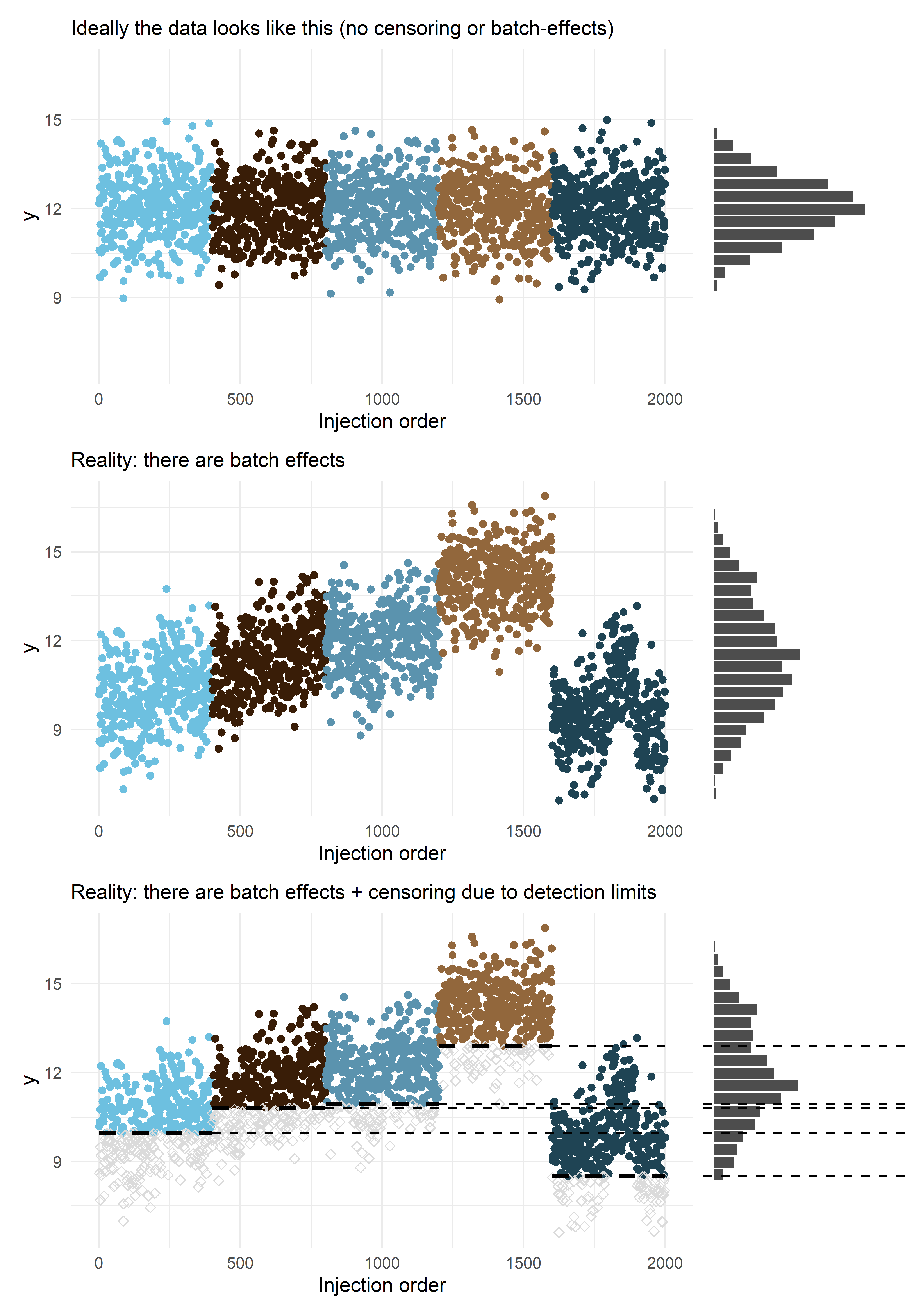
The status quo of imputation and technical variation adjustment
As I tried to illustrate using these plots, technical variation and left-censoring due to limits of detection (LOD) can be significant hurdles in metabolomics analysis. Yet, read method sections in the literature, and you’ll often find they’re treated like an afterthought. If addressed at all, methods sections will often only briefly state: ‘batch effects were removed using ComBat’ (despite ComBat fundamentally ignoring the censored nature of data below the LOD) or ‘data was imputed using methods X or Y’ (referencing imputation techniques like those by Lubin et al. (2004). or Lazar et al. (2016) which focus solely on left-censoring without inherently handling batch effects).
Furthermore, these references to ‘foundational’ imputation methods (like those by Lubin et al. (2004) or Lazar et al. (2016)) typically lack specifics on the exact imputation model; they neither detail which variables were included in the current study’s imputation nor do the original papers offer clear guidance on which should be included (because it wasn’t the goal of those papers). However, this is important for the analyst and the reader to know, as imputation models and the models for the subsequent analysis need to be congenial – meaning the imputation must account for the relationships you intend to study later. The variables included in imputation can matter greatly!
An integrated statistical model (of left-censoring and technical variation)
Moreover, I will argue that the left-censored modeling (and subsequent imputation) and technical variation adjustment should be done in one and the same model because the technical variation and left-censoring are often intertwined. Namely, the same technical factors causing batch-to-batch (or plate-to-plate) shifts in metabolite levels can also influence instrument sensitivity or baseline noise, thereby changing the effective LOD for different batches. This means that you cannot obtain an unbiased estimate of the technical variation without modeling the left-censoring, or the left-censoring without modeling the the technical variation. The higher proportion of nondetects, the worse the bias can get.
In other words, if you adjust for batch effects before imputation (e.g., using methods like ComBat that ignore censoring), you are applying adjustments to data that contains arbitrary placeholders for non-detects (like LOD/2). This distorts the estimation of the batch effect itself. If you impute your nondetects (using a statistical model) before removing possible batch effects, you need to take the batch effect into account to be in line with the observed data. At that point you may as well integrate them all together in one at the same model.
The brms model presented below is a way to implement such a unified model. It models a left-censored outcome with a random intercept term for the batch, and plate, with the plate nested in the batch. For practical purposes, censored observations are assumed to be censored at the minimum detected value of a batch, but you may also model this as a random parameter. After fitting the model, we impute values below the (technical variation adjusted) limit of detection using the original formula specification. Subsequently, we subtract the technical variation from the data (observed values and imputed nondetects).
Importantly, our model – or any model that attempts to identify and remove technical variation – is contingent on sound experimental design; only with sound experimental design can we say that in expectation the batches and plates should have the same (conditional) mean. If you don’t randomize the positions of the samples, supposed technical variation may be real biological variation. In practice, batches and plates are often not perfectly balanced – either by design or because of chance – our method can then easily include the variables that are required to obtain the same (conditional mean) across batches by including them in the formula specification. Hereby we avoid potentially removing variation not related to technical processes of the instrument.
A {brms} model
nr_imputations <- 100
m <- brms::brm(formula = log_y_obs | cens(left_cens) ~ 1 + x + (1|batch_id/plate_nested_coding),
               data = df |> dplyr::mutate(left_cens = censored * -1),
               cores = 4, seed = 2025, refresh = 1000,
               backend = 'cmdstanr')
Running MCMC with 4 parallel chains...
Chain 1 Iteration: 1 / 2000 [ 0%] (Warmup)
Chain 2 Iteration: 1 / 2000 [ 0%] (Warmup)
Chain 3 Iteration: 1 / 2000 [ 0%] (Warmup)
Chain 4 Iteration: 1 / 2000 [ 0%] (Warmup)
Chain 1 Iteration: 1000 / 2000 [ 50%] (Warmup)
Chain 1 Iteration: 1001 / 2000 [ 50%] (Sampling)
Chain 2 Iteration: 1000 / 2000 [ 50%] (Warmup)
Chain 2 Iteration: 1001 / 2000 [ 50%] (Sampling)
Chain 3 Iteration: 1000 / 2000 [ 50%] (Warmup)
Chain 3 Iteration: 1001 / 2000 [ 50%] (Sampling)
Chain 4 Iteration: 1000 / 2000 [ 50%] (Warmup)
Chain 4 Iteration: 1001 / 2000 [ 50%] (Sampling)
Chain 3 Iteration: 2000 / 2000 [100%] (Sampling)
Chain 3 finished in 60.2 seconds.
Chain 1 Iteration: 2000 / 2000 [100%] (Sampling)
Chain 1 finished in 60.4 seconds.
Chain 2 Iteration: 2000 / 2000 [100%] (Sampling)
Chain 2 finished in 63.3 seconds.
Chain 4 Iteration: 2000 / 2000 [100%] (Sampling)
Chain 4 finished in 66.3 seconds.
All 4 chains finished successfully.
Mean chain execution time: 62.5 seconds.
Total execution time: 66.4 seconds.total_nr_draws <- brms::ndraws(m)
samples_to_draw <- sort(sample(total_nr_draws, nr_imputations))
sigma_draws <- as.data.frame(m, variable = c("sigma"), draw = samples_to_draw) |> dplyr::pull()
# do not include technical variation in draws (= implicitly removing it)
mu_draws <- brms::posterior_linpred(m, re_formula = NA, draw_ids = samples_to_draw) |> t()
re_draws <- brms::posterior_linpred(m, re_formula = NULL, draw_ids = samples_to_draw) -
brms::posterior_linpred(m, re_formula = NA, draw_ids = samples_to_draw)
re_draws <- t(re_draws)
imputed_sets <- matrix(nrow = length(y), ncol = nr_imputations)
for(i in 1:nr_imputations) {
mu <- mu_draws[, i]
sd <- sigma_draws[i]
batch_effect <- re_draws[, i]
lod_adjusted <- df[['log_lod']] - batch_effect
# draw values below lod (cdf inversion method)
## what percentiles belong to start with these params
unif_lower <- pnorm(-Inf, mu, sd)
unif_upper <- pnorm(lod_adjusted, mu, sd)
## draw random percentiles between lower and upper
rand_perc_interval <- runif(length(mu), unif_lower, unif_upper)
## get value belonging to percentile
imputes <- qnorm(rand_perc_interval, mu, sd)
# remove technical variation from detected values
y_adjusted <- df[['log_y_obs']] - batch_effect
imputed_sets[,i] <- ifelse(df[['censored']], imputes, y_adjusted)
}
r <- tibble::as_tibble(imputed_sets)Below we see that the model has indeed recovered the parameters of the data generating process, and that convergence diagnostics (\(\hat{R}\), Bulk ESS, and Tail ESS) fell within acceptable ranges, suggesting reliable posterior estimates.3 The imputations below the LOD are based on these recovered parameters.
summary(m) Family: gaussian
Links: mu = identity; sigma = identity
Formula: log_y_obs | cens(left_cens) ~ 1 + x + (1 | batch_id/plate_nested_coding)
Data: dplyr::mutate(df, left_cens = censored * -1) (Number of observations: 2000)
Draws: 4 chains, each with iter = 2000; warmup = 1000; thin = 1;
total post-warmup draws = 4000
Multilevel Hyperparameters:
~batch_id (Number of levels: 5)
Estimate Est.Error l-95% CI u-95% CI Rhat Bulk_ESS Tail_ESS
sd(Intercept) 1.96 0.79 0.98 4.07 1.00 1671 2049
~batch_id:plate_nested_coding (Number of levels: 20)
Estimate Est.Error l-95% CI u-95% CI Rhat Bulk_ESS Tail_ESS
sd(Intercept) 0.60 0.12 0.41 0.89 1.00 1306 1809
Regression Coefficients:
Estimate Est.Error l-95% CI u-95% CI Rhat Bulk_ESS Tail_ESS
Intercept 11.42 0.85 9.66 13.04 1.00 1576 1708
x 0.07 0.02 0.02 0.11 1.00 5054 2497
Further Distributional Parameters:
Estimate Est.Error l-95% CI u-95% CI Rhat Bulk_ESS Tail_ESS
sigma 1.01 0.02 0.97 1.05 1.00 5162 2790
Draws were sampled using sample(hmc). For each parameter, Bulk_ESS
and Tail_ESS are effective sample size measures, and Rhat is the potential
scale reduction factor on split chains (at convergence, Rhat = 1).Visually, we can plot one of the imputed sets, and see that it fits well with the ideal data distribution that has the technical variation removed and the nondetects imputed. We imputed multiple times to represent and capture the uncertainty around the exact value of the nondetects4. We can also see that some of the observed values are now under the the original limit of detection. This is because – according to our model – these observations would have been nondetects in a ‘usual’ batch. And vice versa, there are some nondetects that would have been observed in a ‘usual’ batch and are now above the original LOD.
Code
df_imputes <- dplyr::bind_cols(df, r)

p_a <- df_imputes |>
  ggplot(aes(inj_order, V2)) +
  scale_color_manual(values = unname(bluebrown_colors_list)) +
  geom_point(aes(color = batch_id)) +
  geom_point(data = subset(df_imputes, censored),
             aes(x = inj_order, y = V2), shape = 5) +
  labs(x = x_lab, y = y_lab) +
  batch_lod_hline(df_imputes, nr_batches, samples_p_batch,
                  linewidth = linewidth, linetype = 'dashed') +
  ylim(c(min(df$log_y), max(df$log_y))) +
  theme_minimal() +
  theme(legend.position = 'none')

p_b <- df_imputes |>
  ggplot(aes(x = V2)) +
  geom_histogram(bins = nr_bins, fill = 'black', alpha = 0.7, color = 'white') +
  xlim(c(min(df$log_y), max(df$log_y))) +
  ylim(c(0, axis_range_bins)) +
  geom_vline(aes(xintercept = log_lod), linetype = 'dashed', linewidth = linewidth - 0.3) +
  coord_flip() +
  theme_void()

p_a + p_b + plot_layout(ncol = 2, nrow = 1, widths = c(3, 1))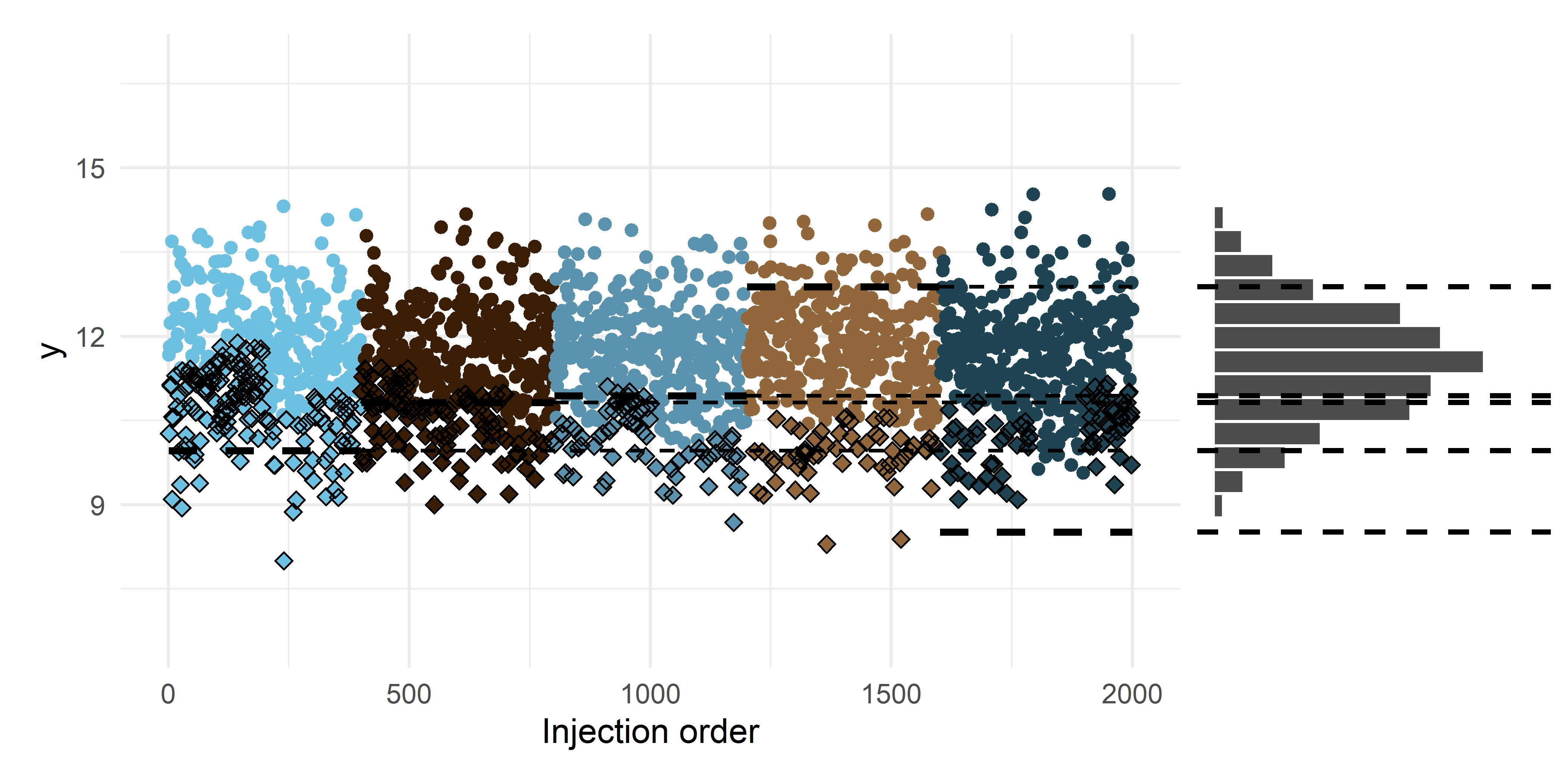
And if we plot the values from an imputed set vs the original values we see the increased uncertainty in values below the LOD:
Code
df_imputes |>
  dplyr::filter(plate_nested_coding == '4_4') |>
  ggplot(aes(V2, log_y, color = censored)) +
  geom_point() +
  geom_hline(aes(yintercept = log_lod), linetype = 'dashed') +
  see::scale_color_okabeito(order = c(2,1)) +
  labs(x = 'Original value', y = 'An imputed set value') +
  theme_minimal()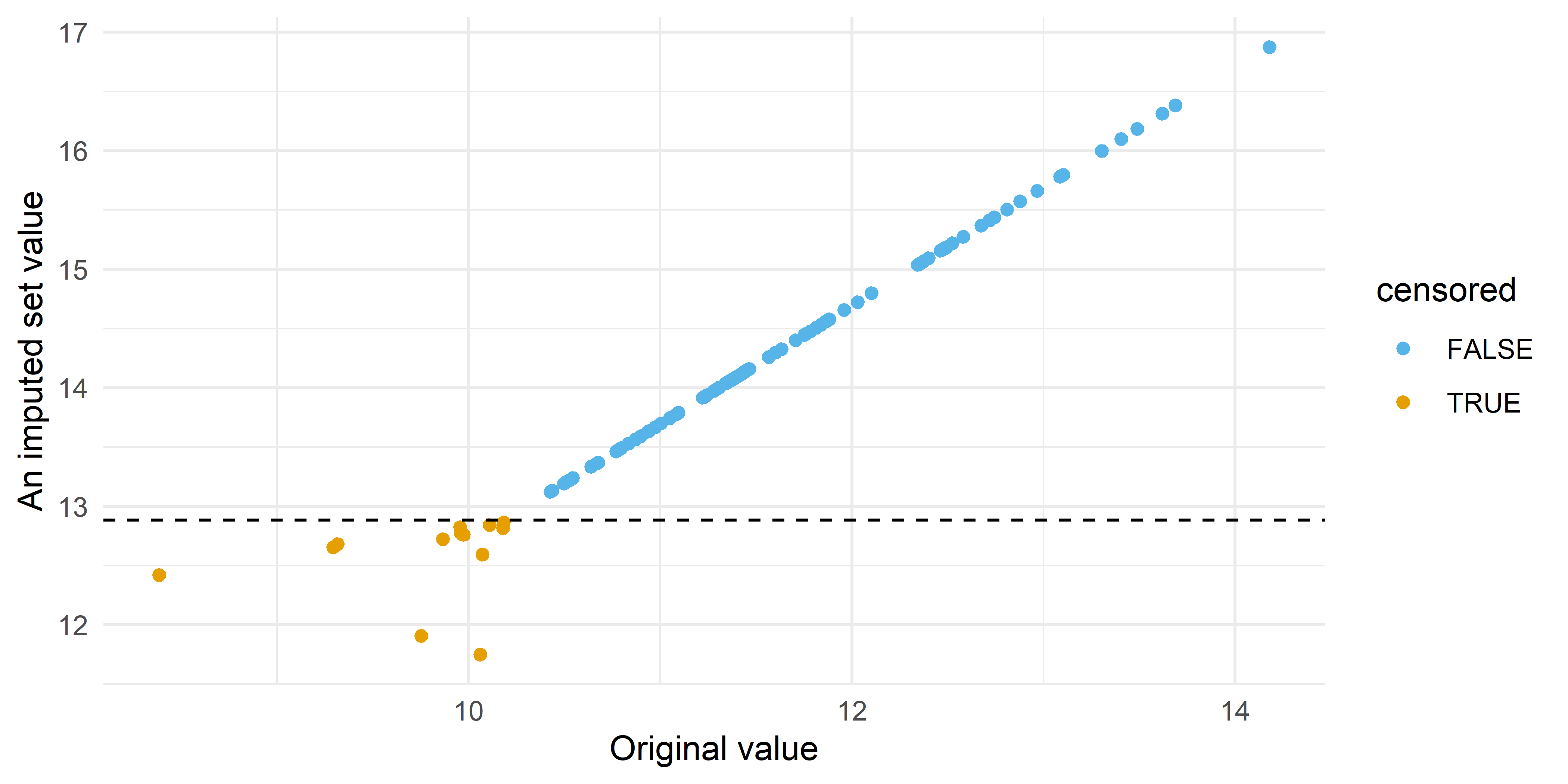
We can also show this by plotting the posterior (100 draws) of a single, imputed, data point below the LOD:
Code
library(magrittr)

df_imputes|>
  tidyr::pivot_longer(starts_with('V')) |>
  dplyr::filter(censored) %>%
  dplyr::filter(inj_order == sample(unique(.$inj_order), 1)) |>
  ggplot(aes(x = value)) +
  ggdist::stat_dotsinterval() +
  labs(x = 'Imputed value') +
  guides(fill = 'none') +
  theme_minimal() +
  theme(axis.title.y = element_blank(),
        axis.text.y = element_blank(), axis.ticks.y = element_blank())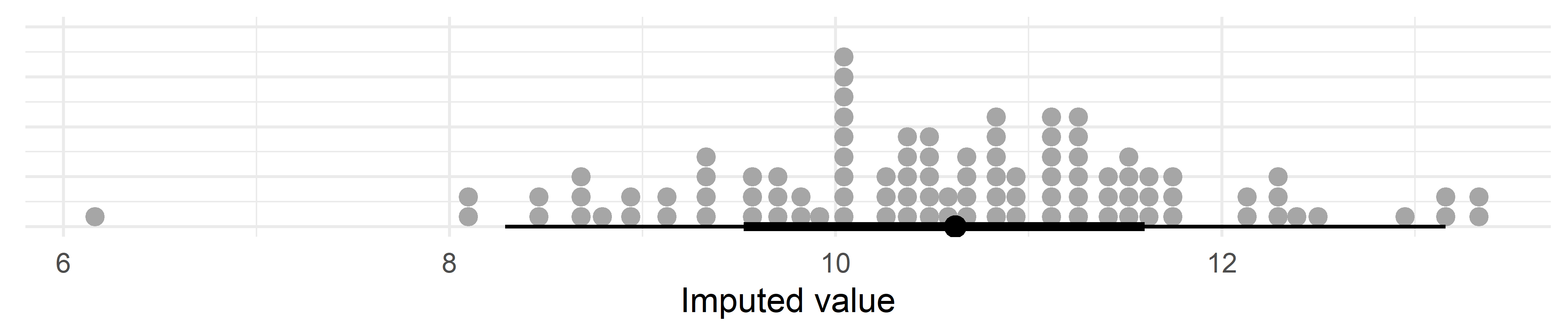
Challenges and solutions (and a two-step model as compromise)
In this exact approach to imputation and technical variation, your imputation and technical variation adjustment needs to be bespoke; you cannot do this imputation and ‘denoising’ once for your dataset and be done with it (if you care to this degree about bias). In theory, you could build the richest possible imputation model (and thus technical variation removal model) that is congenial with the most complex analysis that you would like to do and be done with it. In practice, this would be impossible for labs because they do not have (all) the covariate data, and it would be hard to do for data recipients with the amount of times a dataset is reanalysed by different analysts and the near certainty of missing values for the other variables in a rich imputation model5. It will be even harder to create a congenial dataset when a mixture is the topic of interest and the dataset contains many left-censored features because you would need to impute in two variables simultaneously and it’s not trivial to fit a multivariate left-censored model6.
One potential way around this intertwined nature may be using the pooled QC samples for the batch adjustment using some kind of LOESS fit across the injection order. However, (1) labs do not always deliver information on QCs (2) there are less QC samples than study samples and as such there’s less data to inform such a model (3) readily available LOESS models do not take left-censoring into account. More importantly, it also wouldn’t incorporate other covariates in the adjustment process which risks removing real biological variation and potentially failing to capture that – for example – cases are more often censored. Such a LOESS approach also still separates batch correction from the imputation of study samples, failing to address this interdependence between batch-specific LODs and the imputation process itself.
Another way around this – that is potentially attractive to labs if they also want to provide a batch adjusted dataset – is to slightly change our approach. We still take the intertwined nature of nondetects and batch effects into account by fitting the same statistical model. But contrary to what I described before, we do not impute. We only remove the technical variation by subtracting the technical variation terms from the observed data. We leave the imputation to the analyst. That part can still be bespoke. But the analyst can now just focus on creating a congenial imputation model like they have probably done before for more common epidemiological data. They do not need to worry about the technical variation7. They only need a mice implementation of the left-censored imputation model from Lubin et al. (2004) and they are ready to go – and crucially, within that familiar mice framework they can straightforwardly handle missingness in other covariates alongside the left-censored values. As with the LOESS approach discussed above, the lab will typically not have access to epidemiological covariates when performing this adjustment, meaning structured epidemiological variation risks being misattributed to technical sources and removed – a problem that becomes particularly acute in more complex batch designs involving, for example, blocks or other structured imbalances across batches. I think such a two-step approach is less elegant (as uncertainty in e.g. technical variation is not propagated) and likely less statistically efficient, but it meets a need of many labs and analysts and I think it’s a marked improvement over what they usually do.
In code, this approach would look as follows:
re_draws <- brms::posterior_linpred(m, re_formula = NULL, draw_ids = samples_to_draw) -
  brms::posterior_linpred(m, re_formula = NA, draw_ids = samples_to_draw)

re_summary <- data.frame(
  Estimate = apply(re_draws, 2, mean),
  Est.Error = apply(re_draws, 2, sd),
  Q2.5 = apply(re_draws, 2, quantile, probs = 0.025),
  Q97.5 = apply(re_draws, 2, quantile, probs = 0.975)
)

df$mean_re_estimate <- re_summary$Estimate
df$log_y_adjusted <- df$log_y_obs - df$mean_re_estimate
Just to illustrate the adjusted, non-imputed data we are moving forward with now:
Code
p_c <- df |>
  ggplot(aes(inj_order, log_y_adjusted)) +
  scale_color_manual(values = unname(bluebrown_colors_list)) +
  geom_point(aes(color = batch_id)) +
  geom_point(data = subset(df, censored),
             aes(x = inj_order, y = log_y_adjusted), shape = 5) +
  labs(x = x_lab, y = y_lab) +
  batch_lod_hline(df, nr_batches, samples_p_batch,
                  linewidth = linewidth, linetype = 'dashed') +
  ylim(c(min(df$log_y), max(df$log_y))) +
  theme_minimal() +
  theme(legend.position = 'none')

p_d <- df |>
  ggplot(aes(x = log_y_adjusted)) +
  geom_histogram(bins = nr_bins, fill = 'black', alpha = 0.7, color = 'white') +
  xlim(c(min(df$log_y), max(df$log_y))) +
  ylim(c(0, axis_range_bins)) +
  geom_vline(aes(xintercept = log_lod), linetype = 'dashed', linewidth = linewidth - 0.3) +
  coord_flip() +
  theme_void()

p_c + p_d + plot_layout(ncol = 2, nrow = 1, widths = c(3, 1))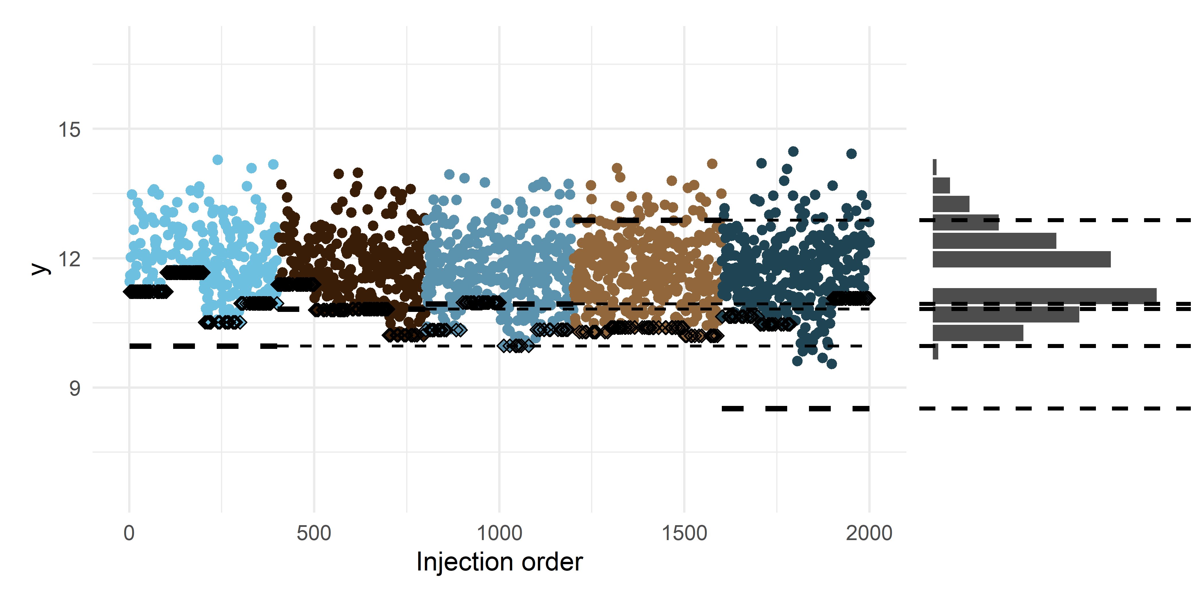
And then we can setup these functions to work with mice:
mice.impute.tobit <- function(y, ry, x, wy = NULL, lod = NULL, ...) {
  # parent trick via
  # github.com/alexpkeil1/qgcomp/blob/2d0c995c0e5117f927ba775f6ee04901f678a7c7/R/base_extensions.R
  whichvar <- eval(as.name("j"), parent.frame(n = 2))
  nms <- names(eval(as.name("data"), parent.frame(n = 3)))
  j <- which(nms == whichvar)
  lod1 <- lod[[j]]
  y1 <- y
  y1[wy] <- lod1[wy]

  m <- survival::survreg(survival::Surv(y1, ry, type = 'left') ~ x, dist = "gaussian")
  imputations <- draw_values_interval(mu = predict(m), sd = m$scale, -Inf, lod1)
  imputations_1 <- imputations[wy]
}

# (past code imputation wrapped in function)
# random sampling from a truncated normal variable via the cdf inversion method
# (also known as inverse transform sampling)
draw_values_interval <- function(mu, sd, start, end) {
  # what percentiles belong to start value with these params
  unif_lower <- pnorm(start, mu, sd)
  # what percentiles belong to end value with these params
  unif_upper <- pnorm(end,  mu, sd)
  # draw random percentiles between lower and upper
  rand_perc_interval <- runif(length(mu),  unif_lower, unif_upper)
  # get value belonging to percentile
  drawn_values <- qnorm(rand_perc_interval, mu, sd)
  return(drawn_values)
}

library(mice)

# other variables with missings can readily be added here in the usual fashion
run_mice <- function(df) {
  df_mice  <- df |> dplyr::mutate(log_y = ifelse(censored, NA, log_y))

  dry_miced <- mice::mice(data = df_mice,
                          method = c(rep("", 5), "tobit", ""),
                          lod = c(rep("", 5), list(df_mice$lod), ""),
                          debug = FALSE,
                          print = FALSE,
                          m = 10,
                          maxit = 0, seed = 2025)

  dry_miced$predictorMatrix[] <- 0
  dry_miced$predictorMatrix["log_y", "x"] <- 1

  miced <- mice::mice(data = df_mice,
                      method = c(rep("", 5), "tobit", ""),
                      lod = c(rep("", 5), list(df_mice$lod), ""),
                      predictorMatrix = dry_miced$predictorMatrix,
                      debug = FALSE,
                      print = FALSE,
                      m = 10,
                      maxit = 10, seed = 2025)
}
And then call it as follows:
lods <- df |>
  dplyr::group_by(batch_id, plate_id) |>
  dplyr::summarize(lod = min(log_y_adjusted))

df_mice <- df |>
  dplyr::select(inj_order, batch_id, plate_id, censored, x, log_y = log_y_adjusted) |>
  dplyr::left_join(lods)

miced <- run_mice(df_mice)
And judging by these plots it has produced similar imputed data on the surface level:
Code
miced_c <- complete(miced) |> tibble::as_tibble()
p_e <- miced_c |>
  ggplot(aes(inj_order, log_y)) +
  scale_color_manual(values = unname(bluebrown_colors_list)) +
  geom_point(aes(color = batch_id)) +
  geom_point(data = subset(miced_c, censored),
             aes(x = inj_order, y = log_y), shape = 5) +
  labs(x = x_lab, y = y_lab) +
  batch_lod_hline(df, nr_batches, samples_p_batch,
                  linewidth = linewidth, linetype = 'dashed') +
  ylim(c(min(df$log_y), max(df$log_y))) +
  theme_minimal() +
  theme(legend.position = 'none')

p_f <- miced_c |>
  ggplot(aes(x = log_y)) +
  geom_histogram(bins = nr_bins, fill = 'black', alpha = 0.7, color = 'white') +
  xlim(c(min(df$log_y), max(df$log_y))) +
  ylim(c(0, axis_range_bins)) +
  geom_vline(data = df, aes(xintercept = log_lod), linetype = 'dashed', linewidth = linewidth - 0.3) +
  coord_flip() +
  theme_void()

p_e + p_f + plot_layout(ncol = 2, nrow = 1, widths = c(3, 1))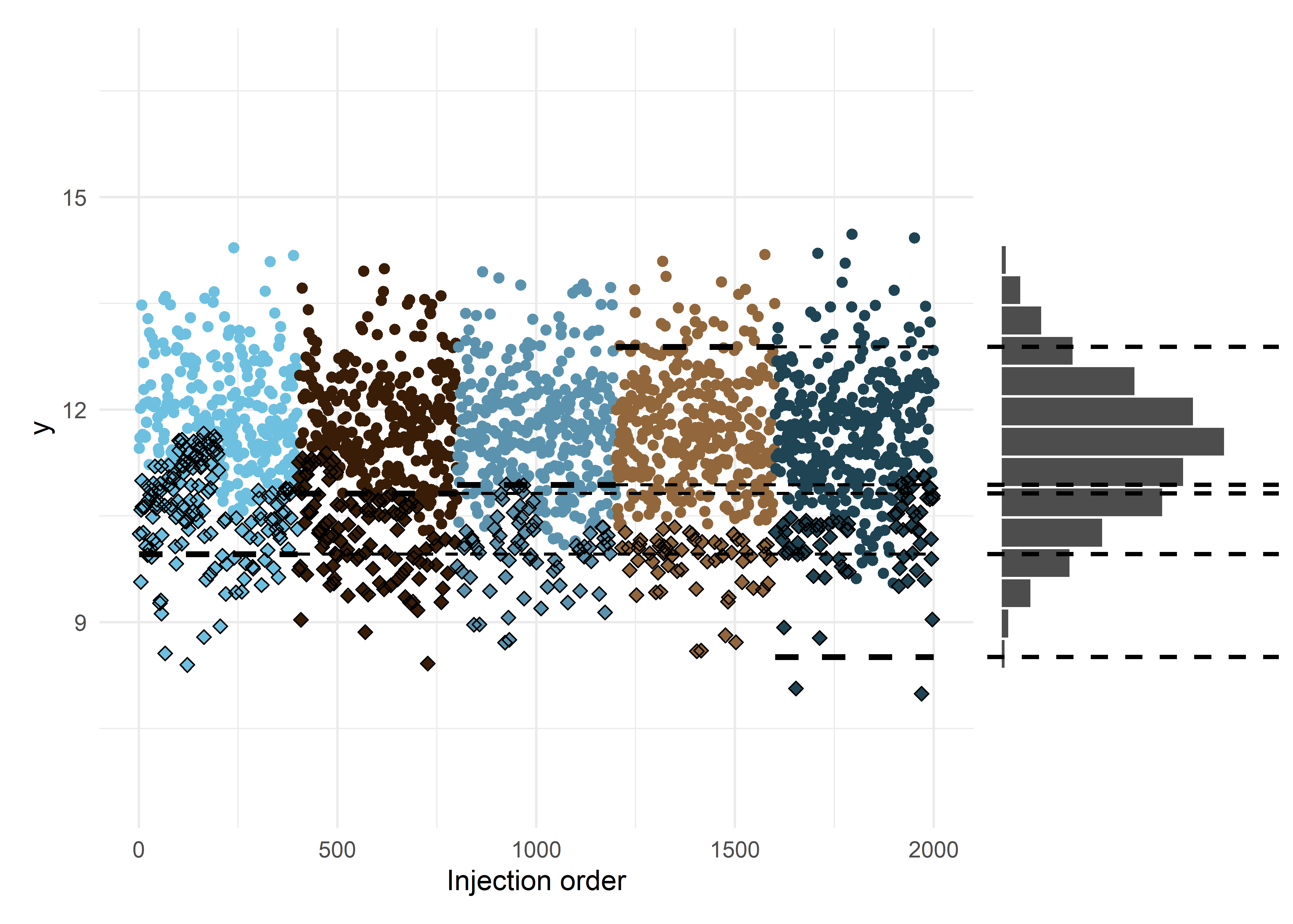
Possible extensions
Sometimes there’s also drift within a plate or a technical variation beyond the batch/plate effects described here. One possible way to model this is by adding a random slope for injection order within a batch or plate. The code from above readily supports this because the code assumes all the random effects are nuisance variation. However, you may want to represent this drift in another way because I think that such more complicated models are much harder to fit. You can consider using some fixed effects8 and then remove their effect using some model.matrix() operation (to keep the effect of variables like e.g. case).
Besides the mean, the variance can be affected by the same processes that introduce technical variation in the mean of batches. We have not modeled that here, but ComBat for example, does model the impact of technical variation on the variance of the batches. We can also take that into account because brms allows you to model the variance as a function of variables. But I imagine that for fitting those models (at scale) you probably want to pool information on this variance parameter across many features in some some hierarchical model or empirical Bayes method (like ComBat).
One final point that I want to make on these models, is on the assumption of a multiplicative error term – here made by the log transformation – in metabolomic data. It’s a useful model in the sense that it permits only positive values (on the original scale) and it is in line with our idea of the data generation process. Namely, it is plausible that the true error structure arises from such a multiplicative process, because measured intensity/concentration can be thought of as a function of duration of exposure \(\times\) number of times exposed. However, in a lognormal distribution the error is also smaller for smaller values. And this is of course opposite of the limit of detection idea. If the error were indeed smaller for smaller values there would be no limit of detection! I hope the multiple versions of the imputed dataset at least overcome this partially. Senn, Holford, and Hockey (2012) mention that realistic likelihood models could consider a complex mixture of true concentration and error measurement models, or model the mean and variance structures separately. While I always like to think about the ideal model, I think for large scale metabolomics – where you often have to fit this model to thousands of features – this is not feasible.
References
Lazar, Cosmin et al. 2016. “Accounting for the Multiple Natures of Missing Values in Label-Free Quantitative Proteomics Data Sets to Compare Imputation Strategies.” Journal of Proteome Research 15 (4): 1116–25. doi:10.1021/acs.jproteome.5b00981.
Lubin, Jay H. et al. 2004. “Epidemiologic Evaluation of Measurement Data in the Presence of Detection Limits.” Environmental Health Perspectives 112 (17): 1691–96. doi:10.1289/ehp.7199.
Senn, Stephen, Nick Holford, and Hans Hockey. 2012. “The Ghosts of Departed Quantities: Approaches to Dealing with Observations Below the Limit of Quantitation.” Statistics in Medicine 31 (30). Wiley Online Library: 4280–95. doi:10.1002/sim.5515.
Footnotes
Also known as nontargeted.↩︎
If your research question pertains directly to the exposure or metabolite level itself – rather than its relationship as a predictor for an outcome – then imputation is not necessary of course, because you can directly use the fitted left-censored model.↩︎
Depending on the textbook, an \(\hat{R}\) smaller than 1.01 or 1.05 is seen as acceptable. For Effective Sample Size (ESS), the recommendation is at least 100 independent draws per MCMC chain (e.g., a total ESS \(>400\) if running the standard 4 chains). In short: \(\hat{R}\) checks if your different chains mixed well and are in agreement with each other. Bulk ESS tells you if you have enough independent draws to trust the center (mean/median) of your estimates, and Tail ESS confirms you have enough draws to confidently report the extremes (like your 95% credible intervals). Always important to check these (or at least sample some models if you fit many). Standard frequentist frameworks don’t offer these kinds of rich, built-in warnings about whether your parameter estimation actually worked, so it would be a shame to ignore them when you have them!↩︎
In discussions I get the sense that many people think that the goal of imputation in metabolomics is to get as close as possible to the value that we would have observed with unlimited instrument sensitivity. While that’s welcome, for valid downstream inference with censored data it’s more important to accurately represent the uncertainty associated with those unobserved values.↩︎
Although
brmsseems to accommodate this as well. This extension is left as an exercise to the reader.↩︎I think some kind of Gibbs sampler or some chained equation is the best we can do. Update: see this blog post on how to do this.↩︎
Not many people worry about the technical variation anyhow – but now there’s also less need to.↩︎
I’m not fully sure what’s better (in such a setup): a model with random slopes that possibly doesn’t fully converge or some 20 fixed effect interaction terms (with potentially some sparsity inducing horseshoe or LASSO priors). I guess putting (very) strong priors on the random slopes is the most logical option. An empirical Bayes method is also worth considering for this.↩︎
Citation
BibTeX citation:
@online{oosterwegel2025,
  author = {Oosterwegel, Max J.},
  title = {Imputing Nondetects and Removing Technical Variation in
    Left-Censored Metabolomic Data},
  date = {2025-04-28},
  url = {https://maxoosterwegel.com/blog/impute-and-remove-technical-variation-metabolomics/},
  doi = {placeholder},
  langid = {en}
}
For attribution, please cite this work as:
Oosterwegel, Max J. 2025. “Imputing Nondetects and Removing
Technical Variation in Left-Censored Metabolomic Data.” April 28.
doi:placeholder.