library(tidyverse)
library(wesanderson)
library(patchwork)
library(gt)
library(gtExtras)
source("functions_features.R")
source("functions_plotting.R")
# Shared gt theme so every table matches the blog's typography and palette
# (header in the heading navy #1D323E, IBM Plex fonts, subtle striping, and
# tabular/monospaced figures so numeric columns line up).
gt_theme_penalties <- function(gt_tbl) {
out <- gt_tbl |>
gt::opt_table_font(font = "IBM Plex Sans") |>
gt::tab_options(
table.width = gt::pct(100),
table.font.size = gt::px(14),
table.border.top.style = "none",
table.border.bottom.color = "#d9dee1",
heading.align = "left",
heading.title.font.size = gt::px(15),
heading.subtitle.font.size = gt::px(12.5),
column_labels.background.color = "#1D323E",
column_labels.font.weight = "bold",
column_labels.font.size = gt::px(12.5),
column_labels.border.bottom.style = "none",
row.striping.background_color = "#f3f5f6",
table_body.hlines.style = "none",
table_body.border.bottom.color = "#d9dee1",
data_row.padding = gt::px(6),
source_notes.font.size = gt::px(11),
source_notes.padding = gt::px(6)
) |>
gt::opt_row_striping() |>
gt::tab_style(
style = gt::cell_text(color = "white"),
locations = gt::cells_column_labels()
) |>
gt::tab_style(
style = gt::cell_text(font = "IBM Plex Mono"),
locations = gt::cells_body(columns = dplyr::where(is.numeric))
)
# When a table has a spanner, the top header row is otherwise a navy "blob"
# identical to the column labels below it. Give it a distinct, lighter look
# (pale fill, dark normal-weight italic text) so the two header rows read as
# caption-over-labels rather than one solid band. Guarded for spanner-less
# tables, since this theme is applied to all of them.
if (nrow(out[["_spanners"]]) > 0) {
out <- out |>
gt::tab_style(
style = list(
gt::cell_fill(color = "#eef2f4"),
gt::cell_text(color = "#1D323E", weight = "normal", style = "italic", size = gt::px(11))
),
locations = gt::cells_column_spanners()
)
}
out
}
# Readable labels for the compact categorical codes used across the tables.
position_labels <- c(
G = "Goalkeeper",
D = "Defender",
M = "Midfielder",
A = "Attacking midfielder",
F = "Forward",
Sub = "Substitute"
)
label_position <- function(x) {
dplyr::coalesce(unname(position_labels[as.character(x)]), as.character(x))
}
# Split camelCase foul codes and sentence-case them: "AerialFoul" -> "Aerial foul"
label_foul <- function(x) {
x |>
as.character() |>
stringr::str_replace_all("(?<=[a-z])(?=[A-Z])", " ") |>
stringr::str_to_sentence()
}
# "losing_3_plus" -> "Losing 3+", "equal" -> "Equal", "winning_1" -> "Winning 1"
label_game_state <- function(x) {
x |>
as.character() |>
stringr::str_replace("_plus", "+") |>
stringr::str_replace_all("_", " ") |>
stringr::str_to_sentence()
}
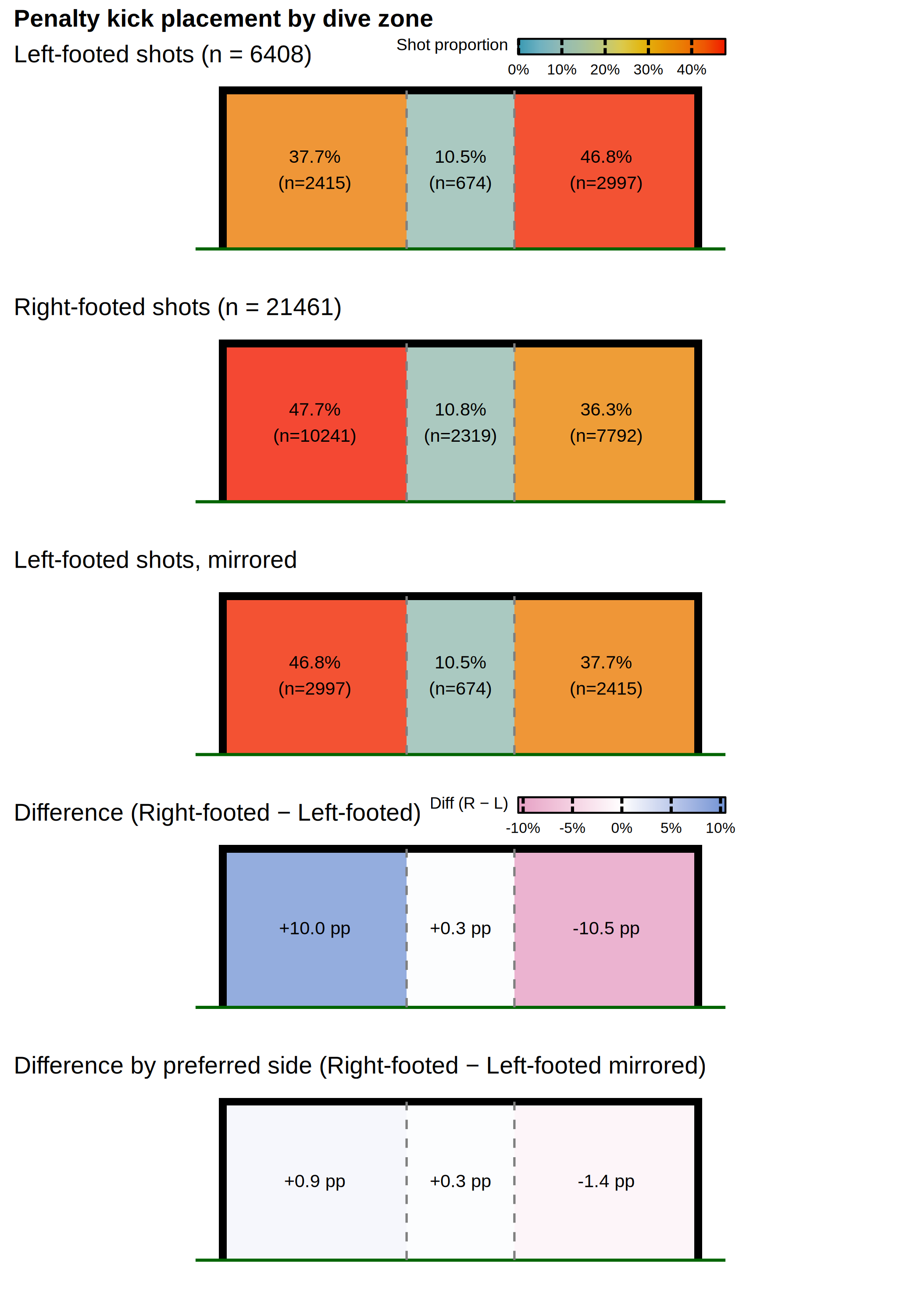
# Shared builder for the placement (shot-zone-dominance) tables. Each row is a
# group (game state, phase, position, experience...) and the three columns
# Dominant/Centre/Non-dominant are that group's placement split, which always
# sums to 100%. Every one of these tables asks a *comparative* question -- "does
# the strong-side preference change ACROSS groups?" -- so the colour highlights
# differences DOWN each column, not the trivial within-row fact that the dominant
# side is biggest. Each zone column is shaded on a diverging scale centred on its
# own median (the "typical" group), reusing the doc's difference-plot palette
# (GrandBudapest2: pink = below typical, periwinkle = above). Centring on the
# median keeps a small, tiny-n outlier group from hijacking the whole scale.
placement_gradient_table <- function(data, group, group_label) {
wide <- data |>
dplyr::filter(!is.na(shot_zone_dominance)) |>
dplyr::select(rowcat = {{ group }}, shot_zone_dominance, prop, prop_n_string) |>
tidyr::pivot_wider(
names_from = shot_zone_dominance,
values_from = c(prop_n_string, prop)
) |>
dplyr::rename(
Dominant = prop_n_string_Dominant,
Centre = prop_n_string_Centre,
Non_dominant = prop_n_string_Non_dominant
) |>
dplyr::relocate(Dominant, Centre, Non_dominant, .after = rowcat)
tbl <- wide |>
gt::gt() |>
gt::tab_spanner(
label = "Shot placement (share of penalties, n)",
columns = c(Dominant, Centre, Non_dominant)
) |>
gt::cols_label(
rowcat = group_label,
Dominant = "Dominant side",
Centre = "Centre",
Non_dominant = "Non-dominant side"
)
# Diverging shading, one column at a time: each zone centred on its own median
# and scaled symmetrically to that column's largest deviation from it.
for (z in c("Dominant", "Centre", "Non_dominant")) {
pcol <- paste0("prop_", z)
vals <- wide[[pcol]]
med <- median(vals, na.rm = TRUE)
spread <- max(abs(vals - med), na.rm = TRUE)
if (is.finite(spread) && spread > 0) {
tbl <- tbl |>
gt::data_color(
columns = dplyr::all_of(pcol),
target_columns = dplyr::all_of(z),
palette = c("#E6A0C4", "#F7F7F5", "#7294D4"),
domain = c(med - spread, med + spread),
na_color = "white"
)
}
}
source_note <- paste(
"Cell colour compares groups down each column:",
"periwinkle = leans on that zone more than the typical (median) group,",
"pink = less. Read the share itself from the cell."
)
tbl |>
gt::cols_hide(c(prop_Dominant, prop_Centre, prop_Non_dominant)) |>
gt::sub_missing(missing_text = "–") |>
gt::tab_source_note(source_note) |>
gt_theme_penalties()
}
df <- nanoparquet::read_parquet(
"data/penalties_ws.parquet"
) |>
convert_opta_to_meters() |>
add_features()
df_male <- df |> dplyr::filter(!is_female_league)
lighten <- function(color, amount = 0.55) {
v <- col2rgb(color) / 255
rgb(
v[1] + (1 - v[1]) * amount,
v[2] + (1 - v[2]) * amount,
v[3] + (1 - v[3]) * amount
)
}
# One base color per subgroup, shades generated within
base_colors <- c(
"Men top 5 league" = "#046C9A", # Darjeeling2 navy
"Men non top level league" = "#78B7C5", # Zissou sky blue (same family, lower tier)
"Men other European league" = "#00A08A", # Darjeeling1 teal-green
"Men league outside Europe" = "#D8B70A", # Cavalcanti gold
"Men cup" = "#F98400", # Darjeeling1 orange
"Men international club" = "#C93312", # Darjeeling2 brick red
"Men international country" = "#9986A5", # IsleofDogs purple-gray
"Women league" = "#F4B5BD", # Moonrise3 blush
"Women international country" = "#7294D4" # GrandBudapest2 periwinkle
)
treemap_data <- df |>
dplyr::group_by(is_female_league, competition_type_detailed, competition, season) |>
dplyr::tally() |>
dplyr::ungroup() |>
dplyr::summarise(
n = sum(n),
season_min = min(season),
season_max = max(season),
.by = c(is_female_league, competition_type_detailed, competition)
) |>
dplyr::mutate(
prop = n / sum(n),
label = paste0(
stringr::str_replace(competition, "-", "\n"),
"\n",
season_min,
"\u2013",
season_max,
"\n",
n,
" (",
scales::percent(prop, accuracy = 0.1),
")"
),
gender = dplyr::if_else(is_female_league, "Women", "Men"),
subgroup = paste(gender, competition_type_detailed),
comp_id = paste(gender, competition)
) |>
dplyr::arrange(subgroup, dplyr::desc(n)) |>
dplyr::mutate(rank_in_subgroup = dplyr::row_number(), .by = subgroup) |>
dplyr::group_by(subgroup) |>
dplyr::mutate(
fill_color = colorRampPalette(
c(base_colors[subgroup[1]], lighten(base_colors[subgroup[1]]))
)(dplyr::n())[rank_in_subgroup]
) |>
dplyr::ungroup()
treemap_data |>
ggplot2::ggplot(ggplot2::aes(area = n, fill = comp_id, label = label, subgroup = subgroup)) +
treemapify::geom_treemap() +
treemapify::geom_treemap_subgroup_border(color = "white", size = 3) +
treemapify::geom_treemap_subgroup_text(
color = "white",
alpha = 0.5,
fontface = "bold",
place = "topleft",
grow = FALSE,
size = 10
) +
treemapify::geom_treemap_text(
color = "white",
place = "centre",
grow = FALSE,
reflow = TRUE,
min.size = 6
) +
ggplot2::scale_fill_manual(
values = setNames(treemap_data$fill_color, treemap_data$comp_id),
guide = "none"
)